Quantity

Quantity#

brainunit generates standard names for units, combining the unit name (e.g. “siemens”) with a prefixes (e.g. “m”), and also generates squared and cubed versions by appending a number. For example, the units “msiemens”, “siemens2”, “usiemens3” are all predefined. You can import these units from the package brainunit – accordingly, an from brainunit import * will result in everything being imported.

We recommend importing only the units you need, to have a cleaner namespace. For example, import brainunit as u and then using u.msiemens instead of msiemens.

import brainunit as u

In the underlying design, Quantity consists of two attributes (mantissa and unit), and the specific value it represents is calculated by the formula below:

\[ \mathrm{value} = \mathrm{mantissa} \times \mathrm{unit.base} ^ \mathrm{unit.scale} * \text{dimension}, \]

where unit.base is the base for this unit (as the base of the exponent) and unit.scale is the scale for this unit (as the integer exponent of base)

A quantity is equivalent to the scientific notation of

\[ \mathrm{mantissa} \times \mathrm{base}^\mathrm{scale} \]

For example, 5 * ms is equivalent to 5 * 10^-3 * s = 5 * 0.001 * s = 0.005 * s.

You can generate a physical quantity by multiplying a scalar or ndarray with its physical unit:

tau = 20 * u.ms
tau

Quantity(20, "ms")

rates = [10, 20, 30] * u.Hz
rates

Quantity([10 20 30], "Hz")

rates = [[10, 20, 30], [20, 30, 40]] * u.Hz
rates

Quantity([[10 20 30]
          [20 30 40]], "Hz")

brainunit will check the consistency of operations on units and raise an error for dimensionality mismatches:

try:
    tau += 1  # ms? second?
except Exception as e:
    print(e)

Cannot calculate 
20 ms += 1, because units do not match: ms != 1

try:
    3 * u.kgram + 3 * u.amp
except Exception as e:
    print(e)

Cannot calculate 
3 kg + 3 A, because units do not match: kg != A

Creating Quantity Instances#

Creating a Quantity object can be accomplished in several ways, categorized based on the type of input used. Here, we present the methods grouped by their input types and characteristics for better clarity.

import jax.numpy as jnp

Scalar and Array Multiplication#

Multiplying a Scalar with a Unit

5 * u.ms

Quantity(5, "ms")

Multiplying a Jax nunmpy value type with a Unit:

jnp.float64(5) * u.ms

/opt/hostedtoolcache/Python/3.14.4/x64/lib/python3.14/site-packages/jax/_src/numpy/scalar_types.py:55: UserWarning: Explicitly requested dtype float64 requested in asarray is not available, and will be truncated to dtype float32. To enable more dtypes, set the jax_enable_x64 configuration option or the JAX_ENABLE_X64 shell environment variable. See https://github.com/jax-ml/jax#current-gotchas for more.
  return asarray(x, dtype=self.dtype)

Quantity(5., "ms")

Multiplying a Jax numpy array with a Unit:

jnp.array([1, 2, 3]) * u.ms

Quantity([1 2 3], "ms")

Multiplying a List with a Unit:

[1, 2, 3] * u.ms

Quantity([1 2 3], "ms")

Direct Quantity Creation#

Creating a Quantity Directly with a Value

u.Quantity(5)

Quantity(5)

Creating a Quantity Directly with a Value and Unit

u.Quantity(5, unit=u.ms)

Quantity(5, "ms")

Creating a Quantity with a Jax numpy Array of Values and a Unit

u.Quantity(jnp.array([1, 2, 3]), unit=u.ms)

Quantity([1 2 3], "ms")

Creating a Quantity with a List of Values and a Unit

u.Quantity([1, 2, 3], unit=u.ms)

Quantity([1 2 3], "ms")

Creating a Quantity with a List of Quantities

u.Quantity([500 * u.ms, 1 * u.second])

Quantity([ 500. 1000.], "ms")

Using the with_units Method

u.Quantity.with_unit(jnp.array([0.5, 1]), unit=u.second)

Quantity([0.5 1. ], "s")

Unitless Quantity#

Quantities can be unitless, which means they have no units. If there is no unit provided, the quantity is assumed to be unitless. The following are examples of creating unitless quantities:

u.Quantity([1, 2, 3])

Quantity([1 2 3])

u.Quantity(jnp.array([1, 2, 3]))

Quantity([1 2 3])

u.Quantity([])

Quantity([])

Illegal Quantity Creation#

The following are examples of illegal quantity creation:

try:
    u.Quantity([500 * u.ms, 1])
except Exception as e:
    print(e)

All elements must have the same units, but got [Unit("ms"), Unit("1")]

try:
    u.Quantity(["some", "nonsense"])
except Exception as e:
    print(e)

Value 'some' with dtype <U4 is not a valid JAX array type. Only arrays of numeric types are supported by JAX.

try:
    u.Quantity([500 * u.ms, 1 * u.volt])
except Exception as e:
    print(e)

All elements must have the same units, but got [Unit("ms"), Unit("V")]

Creating Functions#

You can create functions that return quantities. The following are examples of creating functions that return quantities:

`brainunit.math.array` & `brainunit.math.asarray`#

Convert the input to a quantity or array.

If unit is provided, the input will be checked whether it has the same unit as the provided unit. (If they have same unit but different scale, the input will be converted to the provided unit.) If unit is not provided, the input will be converted to an array.

u.math.asarray([1, 2, 3])                       # return a jax.Array

Array([1, 2, 3], dtype=int32)

# check if the input has the same unit as the provided unit
u.math.asarray([1, 2, 3] * u.second, unit=u.second)    # return a Quantity

Quantity([1 2 3], "s")

# Same unit, but different scale
u.math.asarray([1, 2, 3] * u.msecond, unit=u.second)    # return a Quantity

Quantity([0.001 0.002 0.003], "s")

# fails because the input has a different unit
try:
    u.math.asarray([1 * u.second, 2 * u.second], unit=u.ampere)
except Exception as e:
    print(e)

Cannot convert to a unit with different dimensions. (units are s and A).

More Functions#

Other functions that can be used to create quantities are:

brainunit.math.arange
brainunit.math.array_spilt
brainunit.math.linespace
brainunit.math.logspace
brainunit.math.meshgrid
brainunit.math.vandermode
Can use with Quantity
- brainunit.math.full
- brainunit.math.empty
- brainunit.math.ones
- brainunit.math.zeros
- brainunit.math.full_like
- brainunit.math.empty_like
- brainunit.math.ones_like
- brainunit.math.zeros_like
- brainunit.math.fill_diagonal
Can use with unit keyword
- brainunit.math.eye
- brainunit.math.identity
- brainunit.math.tri
- brainunit.math.diag
- brainunit.math.tril
- brainunit.math.triu

See the Array Creation Documentation for more information.

Converting to Different Units#

You can convert a quantity to a different unit using the to_decimal method. The following are examples of converting quantities to different units:

q = (1, 2, 3) * u.second
q

Quantity([1 2 3], "s")

q.to_decimal(u.msecond)

Array([1000., 2000., 3000.], dtype=float32, weak_type=True)

brainunit will check the consistency of operations on units and raise an error for dimensionality mismatches:

try:
    q.to_decimal(u.ampere)
except Exception as e:
    print(e)

Cannot convert to the decimal number using a unit with different dimensions. (units are s and A).

Attributes of a Quantity#

The important attributes of a Quantity object are:

mantissa: the mantissa of the quantity
unit: the unit of the quantity
dim: the dimension of the unit of the quantity
ndim: the number of dimensions of quantity’s value
shape: the shape of the quantity’s value
size: the size of the quantity’s value
dtype: the dtype of the quantity’s value

An example#

rates = [[10., 20., 30.], [20., 30., 40.]] * u.Hz
rates

Quantity([[10. 20. 30.]
          [20. 30. 40.]], "Hz")

rates.mantissa

Array([[10., 20., 30.],
       [20., 30., 40.]], dtype=float32)

rates.dim

second ** -1

rates.ndim, rates.shape, rates.size, rates.dtype

(2, (2, 3), 6, dtype('float32'))

Arithmetic Functions#

Like Numpy and Jax numpy, arithmetic operators on arrays apply elementwise.

a = [20, 30, 40, 50] * u.mV
b = jnp.arange(4) * u.mV
b

Quantity([0 1 2 3], "mV")

Addition and Subtraction#

Addition and subtraction of quantities need to have the same units and keep the units in the result.

c = a - b
c

Quantity([20 29 38 47], "mV")

c + b

Quantity([20 30 40 50], "mV")

Multiplication and Division#

Multiplication and division of quantities multiply and divide the values and add and subtract the dimensions of the units.

A = jnp.array([[1, 2], [3, 4]]) * u.mV
B = jnp.array([[5, 6], [7, 8]]) * u.mV

A, B

(Quantity([[1 2]
           [3 4]], "mV"),
 Quantity([[5 6]
           [7 8]], "mV"))

A * B # element-wise multiplication

Quantity([[ 5 12]
          [21 32]], "mV^2")

A @ B # matrix multiplication

Quantity([[19 22]
          [43 50]], "mV^2")

A.dot(B) # matrix multiplication

Quantity([[19 22]
          [43 50]], "mV^2")

A / 2 # divide by a scalar

Quantity([[0.5 1. ]
          [1.5 2. ]], "mV")

if the unit of result is unitless, the unit is removed and returned as jax.Array

A / (2 * u.mV) # divide by a quantity, return jax array

Array([[0.5, 1. ],
       [1.5, 2. ]], dtype=float32)

A / (2 * u.mA) # divide by a quantity, return quantity

Quantity([[0.5 1. ]
          [1.5 2. ]], "ohm")

Power#

The power operator raises the value of the quantity to the power of the scalar, and multiplies the unit by the scalar.

Quantity([[1 2]
          [3 4]], "mV")

A ** 2 # element-wise power

Quantity([[ 1  4]
          [ 9 16]], "mV^2")

Built-in Functions#

brainunit provides a number of built-in functions in Quantity class to perform operations on quantities. These functions are:

unary operations
- positive(+)
- negative(-)
- absolute(abs)
- invert(~)
logical operations
- all
- any
shape operations
- reshape
- resize
- squeeze
- unsqueeze
- spilt
- swapaxes
- transpose
- ravel
- take
- repeat
- diagonal
- trace
mathematical functions
- nonzero
- argmax
- argmin
- argsort
- var
- round
- std
- sum
- cumsum
- cumprod
- max
- mean
- min
- ptp
- clip
- conj
- dot
- fill
- item
- prod
- clamp
- sort

For more details on these functions, refer to the documentation.

Indexing, Slicing and Iterating#

One-dimensional Quantity can be indexed, sliced and iterated over, much like lists and other Python sequences.

a = jnp.arange(10) ** 3 * u.mV
a

Quantity([  0   1   8  27  64 125 216 343 512 729], "mV")

a[2]

Quantity(8, "mV")

a[2:5]

Quantity([ 8 27 64], "mV")

Only same dimension Quantity can be set to a slice of a Quantity.

# equivalent to a[0:6:2] = 1000;
# from start to position 6, exclusive, set every 2nd element to 1000
a[:6:2] = 1000 * u.mV
a

Quantity([1000    1 1000   27 1000  125  216  343  512  729], "mV")

a[::-1] # reversed a

Quantity([ 729  512  343  216  125 1000   27 1000    1 1000], "mV")

for i in a:
    print(i**(1 / 3.))

000001 mV^0.3333333333333333
mV^0.3333333333333333
000001 mV^0.3333333333333333
mV^0.3333333333333333
000001 mV^0.3333333333333333
0000005 mV^0.3333333333333333
0000005 mV^0.3333333333333333
0000005 mV^0.3333333333333333
000001 mV^0.3333333333333333
000001 mV^0.3333333333333333

Multidimensional Quantity can have one index per axis. These indices are given in a tuple separated by commas:

def f(x, y):
    return 10 * x + y
b = jnp.fromfunction(f, (5, 4), dtype=jnp.int32) * u.mV
b

Quantity([[ 0  1  2  3]
          [10 11 12 13]
          [20 21 22 23]
          [30 31 32 33]
          [40 41 42 43]], "mV")

b[2, 3]

Quantity(23, "mV")

b[0:5, 1]  # each row in the second column of b

Quantity([ 1 11 21 31 41], "mV")

b[:, 1]  # equivalent to the previous example

Quantity([ 1 11 21 31 41], "mV")

b[1:3, :]  # each column in the second and third row of b

Quantity([[10 11 12 13]
          [20 21 22 23]], "mV")

When fewer indices are provided than the number of axes, the missing indices are considered complete slices:

b[-1]

Quantity([40 41 42 43], "mV")

The expression within brackets in b[i] is treated as an i followed by as many instances of : as needed to represent the remaining axes. NumPy also allows you to write this using dots as b[i, …].

The dots (…) represent as many colons as needed to produce a complete indexing tuple. For example, if x is a Quantity with 5 axes, then

x[1, 2, …] is equivalent to x[1, 2, :, :, :],
x[…, 3] to x[:, :, :, :, 3] and
x[4, …, 5, :] to x[4, :, :, 5, :].

c = jnp.array([[[0, 1, 2], [10, 12, 13]], [[100, 101, 102], [110, 112, 113]]]) * u.mV # a 3D array (two stacked 2D arrays)
c.shape

(2, 2, 3)

c[1, ...] # same as c[1, :, :] or c[1]

Quantity([[100 101 102]
          [110 112 113]], "mV")

c[..., 2] # same as c[:, :, 2]

Quantity([[  2  13]
          [102 113]], "mV")

Iterating over multidimensional Quantity is done with respect to the first axis:

for row in b:
    print(row)

[0 1 2 3] mV
[10 11 12 13] mV
[20 21 22 23] mV
[30 31 32 33] mV
[40 41 42 43] mV

Operating on Subsets#

.at method can be used to operate on a subset of the Quantity. The following are examples of operating on subsets of a Quantity:

q = jnp.arange(5.0) * u.mV
q

Quantity([0. 1. 2. 3. 4.], "mV")

q.at[2].add(10 * u.mV)

Quantity([ 0.  1. 12.  3.  4.], "mV")

q.at[10].add(10 * u.mV)  # out-of-bounds indices are ignored

Quantity([0. 1. 2. 3. 4.], "mV")

q.at[20].add(10 * u.mV, mode='clip') # out-of-bounds indices are clipped

Quantity([ 0.  1.  2.  3. 14.], "mV")

q.at[2].get()

Quantity(2., "mV")

q.at[20].get()  # out-of-bounds indices clipped

Quantity(4., "mV")

q.at[20].get(mode='fill')  # out-of-bounds indices filled with NaN

Quantity(nan, "mV")

brainunit will check the consistency of operations on units and raise an error for dimensionality mismatches:

try:
    q.at[2].add(10)
except Exception as e:
    print(e)

Cannot convert to a unit with different dimensions. (units are 1 and mV).

brainunit also allows customized fill values for the at method:

q.at[20].get(mode='fill', fill_value=-1 * u.mV)  # custom fill value

Quantity(-1., "mV")

try:
    q.at[20].get(mode='fill', fill_value=-1)
except Exception as e:
    print(e)

Cannot convert to a unit with different dimensions. (units are 1 and mV).

Plotting Quantities#

Quantity objects can be conveniently plotted using Matplotlib. This feature will be turned on automatically if Matplotlib is installed. The following are examples of plotting quantities:

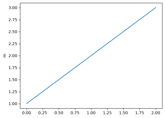
Then Quantity objects can be passed to matplotlib plotting functions. The axis labels are automatically labeled with the unit of the quantity:

from matplotlib import pyplot as plt

plt.figure()
plt.plot([1, 2, 3] * u.meter)

[<matplotlib.lines.Line2D at 0x7fb9f8dec440>]

../_images/c14413569eb94afc735bcc7c9158fc46d443cf9df166a36acc9cd277f980ab8d.png

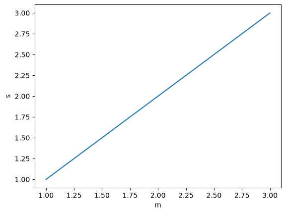
plt.plot([1, 2, 3] * u.meter, [1, 2, 3] * u.second)

[<matplotlib.lines.Line2D at 0x7fb9f8c3ecf0>]

../_images/81c0d890d20ce74fe094ca3795d42218f912ca63c9e27768c4a7ba08a3c4fca5.png

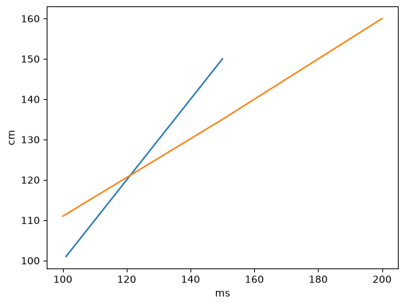
brainunit also supports plotting different scales of quantities with same unit on the same axis:

plt.plot([101, 125, 150] * u.ms, [101, 125, 150] * u.cmeter)
plt.plot([0.1, 0.15, 0.2] * u.second, [111, 135, 160] * u.cmeter)

[<matplotlib.lines.Line2D at 0x7fb9f8b712b0>]

../_images/e13ca0613e622f742618fdce9d392f147cb372f9a139531b8fddc3c795604b92.png

It is not allowed to plot quantities with different units on the same axis:

try:
    plt.plot([101, 125, 150] * u.ms, [101, 125, 150] * u.cmeter)
    plt.plot([0.1, 0.15, 0.2] * u.second, [111, 135, 160] * u.cmeter)
    plt.plot([0.1, 0.15, 0.2] * u.second, [131, 155, 180] * u.mA)
except Exception as e:
    print(e)

Failed to convert value(s) to axis units: Quantity([131 155 180], "mA")

Quantity

Contents

Quantity#

Creating Quantity Instances#

Scalar and Array Multiplication#

Direct Quantity Creation#

Unitless Quantity#

Illegal Quantity Creation#

Creating Functions#

brainunit.math.array & brainunit.math.asarray#

More Functions#

Converting to Different Units#

Attributes of a Quantity#

An example#

Arithmetic Functions#

Addition and Subtraction#

Multiplication and Division#

Power#

Built-in Functions#

Indexing, Slicing and Iterating#

Operating on Subsets#

Plotting Quantities#

`brainunit.math.array` & `brainunit.math.asarray`#