Matplotlib Integration

brainunit integrates with Matplotlib so you can plot Quantity arrays directly. The converter is registered automatically when brainunit is imported, so axis labels show the correct unit name without manual formatting.

import matplotlib.pyplot as plt
import numpy as np

import brainunit as u

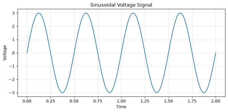
Basic Plotting with Quantities

Pass Quantity arrays directly to plt.plot(). Matplotlib automatically extracts the numeric values and labels axes with units.

t = np.linspace(0.0, 2.0, 200) * u.second
voltage = (3.0 * u.volt) * np.sin(2.0 * np.pi * 2.0 * t.to_decimal(u.second))

fig, ax = plt.subplots(figsize=(8, 4))
ax.plot(t, voltage)
ax.set_xlabel('Time')
ax.set_ylabel('Voltage')
ax.set_title('Sinusoidal Voltage Signal')
ax.grid(alpha=0.3)
plt.tight_layout()
plt.show()

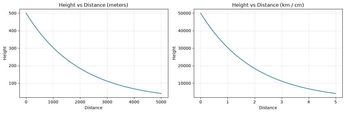
Plotting with Unit Conversion

Use .to() or .in_unit() to convert quantities to different units before plotting.

distance = np.linspace(0, 5000, 100) * u.meter
height = (500.0 * u.meter) * np.exp(-distance.to_decimal(u.meter) / 2000.0)

fig, (ax1, ax2) = plt.subplots(1, 2, figsize=(12, 4))

# Plot in meters
ax1.plot(distance, height)
ax1.set_xlabel('Distance')
ax1.set_ylabel('Height')
ax1.set_title('Height vs Distance (meters)')
ax1.grid(alpha=0.3)

# Plot in kilometers
ax2.plot(distance.in_unit(u.kmeter), height.in_unit(u.cmeter))
ax2.set_xlabel('Distance')
ax2.set_ylabel('Height')
ax2.set_title('Height vs Distance (km / cm)')
ax2.grid(alpha=0.3)

plt.tight_layout()
plt.show()

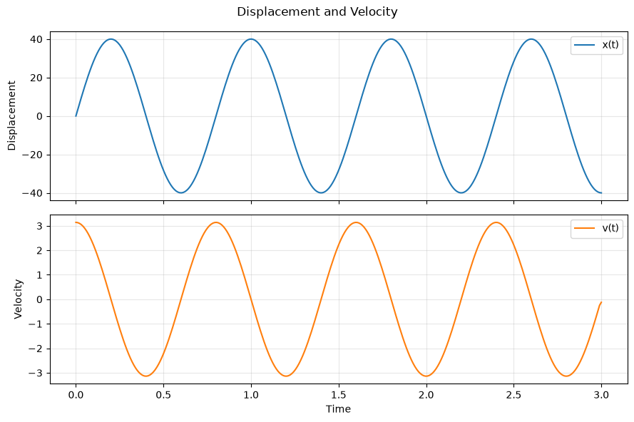
Multiple Signals with Different Units

Use subplots to show related physical quantities with their respective units.

t = np.linspace(0.0, 3.0, 300) * u.second

# Displacement (cm)
x = (40.0 * u.cmeter) * np.sin(2.0 * np.pi * 1.25 * t.to_decimal(u.second))

# Velocity from numerical derivative
v = (
    np.gradient(x.to_decimal(u.meter), t.to_decimal(u.second))
    * (u.meter / u.second)
)

fig, (ax1, ax2) = plt.subplots(2, 1, figsize=(9, 6), sharex=True)

ax1.plot(t, x, label='x(t)')
ax1.set_ylabel('Displacement')
ax1.legend()
ax1.grid(alpha=0.3)

ax2.plot(t, v, color='tab:orange', label='v(t)')
ax2.set_xlabel('Time')
ax2.set_ylabel('Velocity')
ax2.legend()
ax2.grid(alpha=0.3)

fig.suptitle('Displacement and Velocity')
plt.tight_layout()
plt.show()

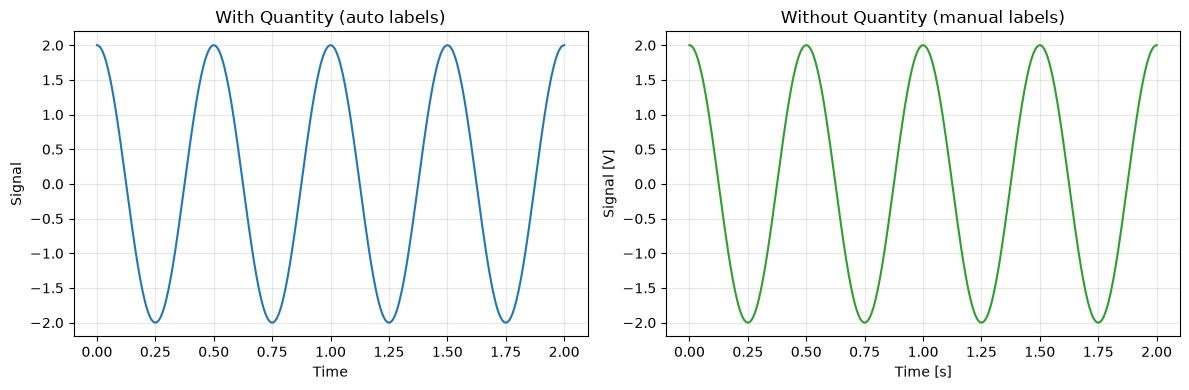
Quantity-Aware vs Plain Numeric

Compare plotting with Quantity (automatic labels) vs plain arrays (manual labels).

t_q = np.linspace(0.0, 2.0, 400) * u.second
y_q = (2.0 * u.volt) * np.cos(2.0 * np.pi * 2.0 * t_q.to_decimal(u.second))

t_plain = t_q.to_decimal(u.second)
y_plain = y_q.to_decimal(u.volt)

fig, (ax1, ax2) = plt.subplots(1, 2, figsize=(12, 4))

# With Quantity: unit labels added automatically
ax1.plot(t_q, y_q, color='tab:blue')
ax1.set_title('With Quantity (auto labels)')
ax1.set_xlabel('Time')
ax1.set_ylabel('Signal')
ax1.grid(alpha=0.3)

# Plain arrays: you must add unit labels manually
ax2.plot(t_plain, y_plain, color='tab:green')
ax2.set_title('Without Quantity (manual labels)')
ax2.set_xlabel('Time [s]')
ax2.set_ylabel('Signal [V]')
ax2.grid(alpha=0.3)

plt.tight_layout()
plt.show()

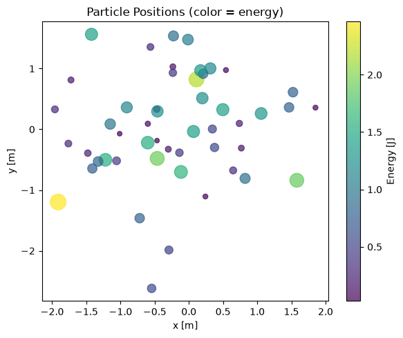
Scatter Plots

# Random particle positions and energies
np.random.seed(42)
x_pos = np.random.randn(50) * u.meter
y_pos = np.random.randn(50) * u.meter
energy = np.abs(np.random.randn(50)) * u.joule

fig, ax = plt.subplots(figsize=(6, 5))
sc = ax.scatter(
    x_pos.to_decimal(u.meter),
    y_pos.to_decimal(u.meter),
    c=energy.to_decimal(u.joule),
    s=energy.to_decimal(u.joule) * 100 + 20,
    alpha=0.7,
    cmap='viridis'
)
ax.set_xlabel('x [m]')
ax.set_ylabel('y [m]')
ax.set_title('Particle Positions (color = energy)')
plt.colorbar(sc, label='Energy [J]')
plt.tight_layout()
plt.show()

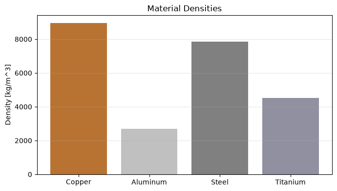
Bar Charts with Physical Quantities

materials = ['Copper', 'Aluminum', 'Steel', 'Titanium']
densities = np.array([8960., 2700., 7850., 4507.]) * u.kilogram / u.meter ** 3

fig, ax = plt.subplots(figsize=(7, 4))
bars = ax.bar(materials, densities.to_decimal(u.kilogram / u.meter ** 3),
              color=['#b87333', '#c0c0c0', '#808080', '#9090a0'])
ax.set_ylabel('Density [kg/m^3]')
ax.set_title('Material Densities')
ax.grid(axis='y', alpha=0.3)
plt.tight_layout()
plt.show()

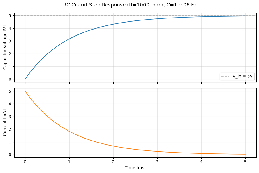
Practical Example: RC Circuit Response

Plot the step response of an RC circuit, where all quantities carry physical units.

# RC circuit parameters
R = 1000.0 * u.ohm  # 1 kohm
C = 1e-6 * u.farad  # 1 uF
V_in = 5.0 * u.volt  # step input

# Time constant
tau = R * C  # ohm * farad = second
print('Time constant (tau):', tau)

# Time array
t = np.linspace(0.0, 5e-3, 500) * u.second

# Voltage across capacitor: V_C(t) = V_in * (1 - exp(-t/tau))
V_cap = V_in * (1 - np.exp(-t.to_decimal(u.second) / tau.to_decimal(u.second)))

# Current: I(t) = V_in/R * exp(-t/tau)
I = (V_in / R) * np.exp(-t.to_decimal(u.second) / tau.to_decimal(u.second))

fig, (ax1, ax2) = plt.subplots(2, 1, figsize=(9, 6), sharex=True)

ax1.plot(t.to_decimal(u.ms), V_cap.to_decimal(u.volt), color='tab:blue')
ax1.axhline(y=5.0, color='gray', linestyle='--', alpha=0.5, label='V_in = 5V')
ax1.set_ylabel('Capacitor Voltage [V]')
ax1.legend()
ax1.grid(alpha=0.3)

ax2.plot(t.to_decimal(u.ms), I.to_decimal(u.mA), color='tab:orange')
ax2.set_xlabel('Time [ms]')
ax2.set_ylabel('Current [mA]')
ax2.grid(alpha=0.3)

fig.suptitle(f'RC Circuit Step Response (R={R}, C={C})')
plt.tight_layout()
plt.show()

Time constant (tau): 0.001 s

How It Works

brainunit automatically registers a QuantityConverter with Matplotlib when imported. This converter:

1. Extracts numeric values from Quantity objects via .mantissa

2. Sets axis labels from the unit’s display name

3. Handles unit conversion if the axis already has a target unit

You can check whether the converter was registered:

from brainunit._matplotlib_compat import matplotlib_converter_registered

print('Matplotlib converter registered:', matplotlib_converter_registered)

---------------------------------------------------------------------------
ModuleNotFoundError                       Traceback (most recent call last)
Cell In[9], line 1
----> 1 from brainunit._matplotlib_compat import matplotlib_converter_registered
      2 
      3 print('Matplotlib converter registered:', matplotlib_converter_registered)

ModuleNotFoundError: No module named 'brainunit._matplotlib_compat'

Tips for Unit-Aware Plotting

Approach	When to Use
Pass Quantity directly	Auto axis labels, simple plots
.to_decimal(unit)	When you need plain arrays for colorbar, custom formatting
.in_unit(unit)	Convert to different unit, keep Quantity for plotting
.to(unit)	Same as .in_unit()