CSR and CSC Sparse Matrices

This chapter treats connectivity as Data: which edges are stored, how their weights are represented, and which orientation matches an operation.

import brainevent
import jax
import jax.numpy as jnp
import matplotlib.pyplot as plt

Why Use Sparse Connectivity Data?

A dense matrix stores every possible edge. CSR and CSC store only explicit nonzero weights plus integer indices. This can reduce storage when connectivity is sparse, but the actual speed and memory benefit depends on shape, sparsity, dtype, operation, backend, and compilation state.

COO Input, CSR Storage, and CSC Storage

Coordinate (COO) data lists (row, column, value) triplets. CSR groups entries by row through indptr; CSC groups them by column. CSR naturally supports row-oriented access and events @ weights; CSC is useful when column-oriented access is primary.

dense = jnp.array([[0.0, 0.5, 0.0, -0.2],
                   [0.3, 0.0, 0.0, 0.0],
                   [0.0, 0.1, 0.4, 0.0]])
csr = brainevent.CSR.fromdense(dense)
csc = brainevent.CSC.fromdense(dense)
print(csr.indptr, csr.indices, csr.data)
print(csc.indptr, csc.indices, csc.data)

[0 2 3 5] [1 3 0 1 2] [ 0.5 -0.2  0.3  0.1  0.4]
[0 1 3 4 5] [1 0 2 2 0] [ 0.3  0.5  0.1  0.4 -0.2]

Constructing CSR and CSC Data

fromdense is convenient for small examples. In data pipelines, construct from sparse source data when possible so a large dense intermediate is never materialized. Converting back with todense() is appropriate for validation and visualization at small scale.

assert jnp.array_equal(csr.todense(), dense)
assert jnp.array_equal(csc.todense(), dense)
print(csr.shape, csc.shape, csr.nse)

(3, 4) (3, 4) 5

Combining Sparse Data with Binary Events

The sparse object describes connectivity; BinaryArray describes active presynaptic events. Keeping those responsibilities separate makes the same connectivity reusable with binary or dense activity.

events = brainevent.BinaryArray(jnp.array([True, False, True]))
sparse_output = events @ csr
dense_output = events.value.astype(dense.dtype) @ dense
print(sparse_output)
assert jnp.allclose(sparse_output, dense_output)

[ 0.   0.6  0.4 -0.2]

Memory, Correctness, and Performance

Correctness should be checked separately from performance. The comparison below compiles each path, synchronizes device work, then times one steady-state call. Treat the result as a local measurement, not a general ranking.

from time import perf_counter

sparse_step = jax.jit(lambda x: x @ csr)
dense_step = jax.jit(lambda x: x.value.astype(dense.dtype) @ dense)

sparse_step(events).block_until_ready()
dense_step(events).block_until_ready()
start = perf_counter(); sparse_result = sparse_step(events); sparse_result.block_until_ready(); sparse_seconds = perf_counter() - start
start = perf_counter(); dense_result = dense_step(events); dense_result.block_until_ready(); dense_seconds = perf_counter() - start
assert jnp.allclose(sparse_result, dense_result)
print({'sparse_seconds': sparse_seconds, 'dense_seconds': dense_seconds})

{'sparse_seconds': 0.00037254700001199126, 'dense_seconds': 0.00014423999999735315}

Build a Sparse Event-Driven Network

A layer can reuse one CSR matrix for a batch of event vectors. A two-dimensional BinaryArray performs the batch operation without a Python time-step loop.

event_batch = brainevent.BinaryArray(jnp.array([[1, 0, 1], [0, 1, 0]], dtype=bool))
network_output = event_batch @ csr
print(network_output.shape)
print(network_output)

(2, 4)
[[ 0.   0.6  0.4 -0.2]
 [ 0.3  0.   0.   0. ]]

Inspect the Connectivity Structure

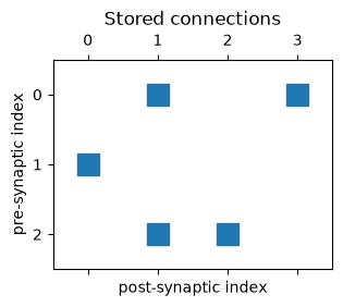
For small matrices, a dense image is a useful structural diagnostic. Avoid materializing large sparse matrices solely for plotting.

fig, ax = plt.subplots(figsize=(5, 2.5))
ax.spy(csr.todense(), markersize=14)
ax.set(xlabel='post-synaptic index', ylabel='pre-synaptic index', title='Stored connections')
plt.show()

Choosing CSR or CSC

Choose by the dominant access direction, not by a universal performance claim. Start with CSR for row-oriented forward event propagation. Prefer CSC when repeated column-oriented operations dominate. Measure the real workload on the intended hardware.

Summary and Next Steps

CSR and CSC encode the same sparse matrix with different orientation. Continue to Fixed Connection Count Structures when every neuron must have a fixed fan-in or fan-out, or to Just-in-Time Connection Matrices when reproducible random connectivity should be generated rather than stored.