Building a Spiking Neural Network

BrainState provides the substrate for brain modeling — State, Module, integrators, delays, and event-driven operators — but it deliberately ships few concrete neuron or synapse models. Those live in the companion package brainpy, whose brainpy.state API is built directly on BrainState. This is the intended cross-package workflow: import ready-made LIF, synapse, and projection models from brainpy.state, and wire them together as ordinary BrainState modules.

We build a classic excitatory–inhibitory (E/I) balanced network one piece at a time, then run it and plot the resulting spike raster.

import brainunit as u
import jax.numpy as jnp
import matplotlib.pyplot as plt

import brainstate
import brainpy
import braintools

brainstate.random.seed(0)
brainstate.environ.set(dt=0.1 * u.ms)
brainstate.__version__

An NVIDIA GPU may be present on this machine, but a CUDA-enabled jaxlib is not installed. Falling back to cpu.

'0.4.0'

Step 1: a population of spiking neurons

brainpy.state.LIF is a leaky integrate-and-fire population — a BrainState Dynamics module. All physical quantities carry units (via brainunit): potentials in millivolts, time constants in milliseconds. After init_all_states, the population is ready to be driven by an input current.

neurons = brainpy.state.LIF(
    4,
    V_rest=-52. * u.mV,
    V_th=-50. * u.mV,
    V_reset=-60. * u.mV,
    tau=10. * u.ms,
    V_initializer=braintools.init.Constant(-60. * u.mV),
    spk_reset='soft',
)
brainstate.nn.init_all_states(neurons)

# Drive the neurons with a constant supra-threshold current for one step.
with brainstate.environ.context(t=0. * u.ms):
    spikes = neurons(8. * u.mA)
print('membrane potential:', neurons.V.value)
print('spikes this step  :', spikes)

membrane potential: [-59.84079742 -59.84079742 -59.84079742 -59.84079742] mV
spikes this step  : [0. 0. 0. 0.]

Step 2: connecting populations with a projection

A projection carries spikes from a source population to a target. We assemble one from four composable parts:

• a communication operator — EventFixedProb, the event-driven sparse connectivity from the previous tutorial;

• a synapse model — Expon, exponential conductance decay;

• an output model — CUBA, current-based synaptic input;

• the postsynaptic population.

brainpy.state.AlignPostProj binds them together. The .desc(...) calls are deferred constructors that the projection instantiates against the target population.

projection = brainpy.state.AlignPostProj(
    comm=brainstate.nn.EventFixedProb(4, 4, conn_num=0.5, conn_weight=1.0 * u.mS),
    syn=brainpy.state.Expon.desc(4, tau=2. * u.ms),
    out=brainpy.state.CUBA.desc(),
    post=neurons,
)
print(type(projection).__name__, 'connects a source onto', neurons.varshape, 'neurons')

AlignPostProj connects a source onto (4,) neurons

Step 3: assembling the E/I network

A balanced network has an excitatory and an inhibitory sub-population, each projecting onto the whole network. We wrap a single LIF population (the first n_exc units are excitatory, the rest inhibitory) and two projections in one Module. Its update reads the current spikes, routes them through the two projections, then advances the neurons by one step.

class EINet(brainstate.nn.Module):
    def __init__(self, n_exc, n_inh, prob, JE, JI):
        super().__init__()
        self.n_exc = n_exc
        self.num = n_exc + n_inh
        self.N = brainpy.state.LIF(
            self.num,
            V_rest=-52. * u.mV, V_th=-50. * u.mV, V_reset=-60. * u.mV,
            tau=10. * u.ms,
            V_initializer=braintools.init.Normal(-60., 10., unit=u.mV),
            spk_reset='soft',
        )
        self.E = brainpy.state.AlignPostProj(
            comm=brainstate.nn.EventFixedProb(n_exc, self.num, prob, JE),
            syn=brainpy.state.Expon.desc(self.num, tau=2. * u.ms),
            out=brainpy.state.CUBA.desc(), post=self.N,
        )
        self.I = brainpy.state.AlignPostProj(
            comm=brainstate.nn.EventFixedProb(n_inh, self.num, prob, JI),
            syn=brainpy.state.Expon.desc(self.num, tau=2. * u.ms),
            out=brainpy.state.CUBA.desc(), post=self.N,
        )

    def update(self, inp):
        spikes = self.N.get_spike() != 0.
        self.E(spikes[:self.n_exc])     # excitatory spikes
        self.I(spikes[self.n_exc:])     # inhibitory spikes
        self.N(inp)                     # advance the neurons
        return self.N.get_spike()

Step 4: running the simulation

We instantiate a 500-neuron network (400 excitatory, 100 inhibitory), initialise its state, and step it for 200 ms under a constant background current. brainstate.transform.for_loop runs the whole trajectory as a single compiled scan, collecting the spikes at every step.

n_exc, n_inh, prob = 400, 100, 0.1
# Balanced weights scale as 1/sqrt(expected number of inputs).
JE = 1. / u.math.sqrt(prob * n_exc) * u.mS
JI = -1. / u.math.sqrt(prob * n_inh) * u.mS

net = EINet(n_exc, n_inh, prob, JE, JI)
brainstate.nn.init_all_states(net)

times = u.math.arange(0. * u.ms, 200. * u.ms, brainstate.environ.get_dt())
spikes = brainstate.transform.for_loop(lambda t: net.update(3. * u.mA), times)
print('spike array shape (time, neurons):', spikes.shape)
print('total spikes:', int(jnp.sum(spikes != 0)))

spike array shape (time, neurons): (2000, 500)

total spikes: 4356

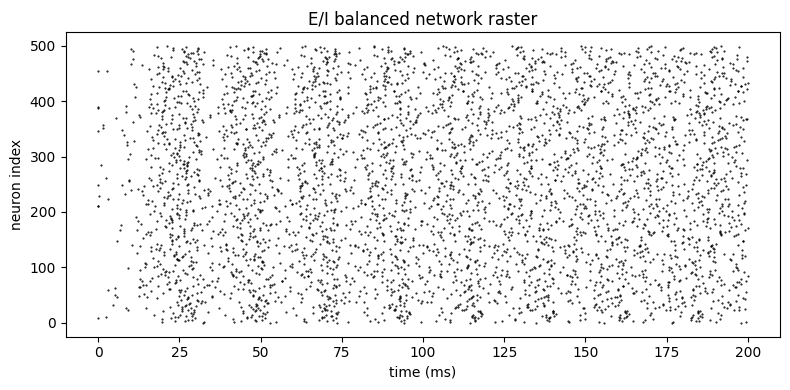
Step 5: the spike raster

A raster plot — neuron index versus spike time — reveals the asynchronous irregular firing characteristic of a balanced network.

t_ms = times.to_decimal(u.ms)
t_idx, n_idx = u.math.where(spikes != 0)

plt.figure(figsize=(8, 4))
plt.plot(t_ms[t_idx], n_idx, 'k.', markersize=1)
plt.xlabel('time (ms)')
plt.ylabel('neuron index')
plt.title('E/I balanced network raster')
plt.tight_layout()
plt.show()

Summary

• BrainState is the substrate; brainpy.state supplies concrete LIF neurons, Expon synapses, CUBA outputs, and AlignPostProj projections, all as BrainState modules.

• A projection composes a communication operator, a synapse, an output, and a postsynaptic population — here using the event-driven EventFixedProb.

• init_all_states prepares a network and brainstate.transform.for_loop runs the trajectory as one compiled scan.

See also

• Training a spiking neural network — making such a network learn with surrogate gradients.

• Event-driven operators — the connectivity used in the projections.

• The brain-dynamics gallery — complete simulation and Hodgkin–Huxley examples.