
Training a Spiking Neural Network#
A spiking network unrolled over time is a recurrent network, so it can be trained with backpropagation through time. The one obstacle is the spike itself: a threshold function has zero gradient almost everywhere, so gradients cannot flow back through it. The standard remedy is a surrogate gradient — use the hard threshold on the forward pass, but a smooth approximation for the backward pass.
This tutorial trains a small spiking classifier end to end: define the network with a surrogate
spike function, generate a synthetic spike dataset, and optimise it with braintools.optim and
brainstate.transform.grad.
import brainunit as u
import jax.numpy as jnp
import matplotlib.pyplot as plt

import brainstate
import brainpy
import braintools

brainstate.random.seed(0)
brainstate.environ.set(dt=1.0 * u.ms)

num_inputs, num_hidden, num_outputs = 100, 4, 2
num_steps, batch_size = 100, 128
brainstate.__version__
An NVIDIA GPU may be present on this machine, but a CUDA-enabled jaxlib is not installed. Falling back to cpu.
'0.4.0'
The network#
The classifier has three stages: an input projection (Linear followed by an Expon synapse), a
recurrent LIF layer, and a readout (Linear into an Expon output). The crucial detail is
spk_fun=braintools.surrogate.ReluGrad() on the LIF layer — this is what makes the spike
differentiable for training. Weights are initialised with braintools.init.
class SNN(brainstate.nn.Module):
    def __init__(self, n_in, n_rec, n_out):
        super().__init__()
        decay = 1 - u.math.exp(-brainstate.environ.get_dt() / (1 * u.ms))
        self.i2r = brainstate.nn.Sequential(
            brainstate.nn.Linear(
                n_in, n_rec,
                w_init=braintools.init.KaimingNormal(scale=7 * decay, unit=u.mA),
                b_init=braintools.init.ZeroInit(unit=u.mA),
            ),
            brainpy.state.Expon(n_rec, tau=10. * u.ms,
                                g_initializer=braintools.init.Constant(0. * u.mA)),
        )
        self.r = brainpy.state.LIF(
            n_rec, tau=20 * u.ms, V_rest=0 * u.mV, V_reset=0 * u.mV, V_th=1. * u.mV,
            spk_fun=braintools.surrogate.ReluGrad(),   # surrogate gradient for the spike
        )
        self.r2o = brainstate.nn.Linear(n_rec, n_out, w_init=braintools.init.KaimingNormal())
        self.o = brainpy.state.Expon(n_out, tau=10. * u.ms,
                                     g_initializer=braintools.init.Constant(0.))

    def update(self, spike):
        # one time step: input projection -> recurrent spikes -> readout
        return self.o(self.r2o(self.r(self.i2r(spike))))

net = SNN(num_inputs, num_hidden, num_outputs)
A synthetic dataset#
Each example is a num_steps x num_inputs array of Poisson spikes; the label is a random binary
class. The data is intentionally trivial — the point is the training mechanics, not the task.
firing_rate = 5 * u.Hz
x_data = brainstate.random.rand(num_steps, batch_size, num_inputs) < firing_rate * brainstate.environ.get_dt()
y_data = u.math.asarray(brainstate.random.rand(batch_size) < 0.5, dtype=int)
print('input spikes:', x_data.shape, '| labels:', y_data.shape)
input spikes: (100, 128, 100) | labels: (128,)
Loss, optimizer, and the training step#
The loss runs the network over all time steps with for_loop, averages the readout over time,
and applies a cross-entropy. The training step re-initialises the network state for each batch,
differentiates the loss with respect to the parameters (backpropagation through time), and
applies an Adam update — the whole thing wrapped in jit.
def accuracy():
    brainstate.nn.init_all_states(net, batch_size=batch_size)
    outs = brainstate.transform.for_loop(net.update, x_data)
    pred = u.math.argmax(u.math.max(outs, axis=0), axis=1)   # max over time, argmax over class
    return float(u.math.mean(pred == y_data))

print(f'accuracy before training: {accuracy():.3f}')
accuracy before training: 0.438
optimizer = braintools.optim.Adam(lr=3e-3)
optimizer.register_trainable_weights(net.states(brainstate.ParamState))

def loss_fn():
    outs = brainstate.transform.for_loop(net.update, x_data)
    outs = u.math.mean(outs, axis=0)
    return braintools.metric.softmax_cross_entropy_with_integer_labels(outs, y_data).mean()

@brainstate.transform.jit
def train_step():
    brainstate.nn.init_all_states(net, batch_size=batch_size)
    grads, loss = brainstate.transform.grad(
        loss_fn, net.states(brainstate.ParamState), return_value=True)()
    optimizer.update(grads)
    return loss
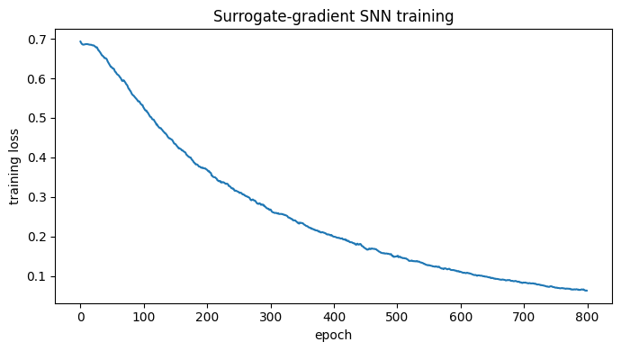
Training#
Each call to train_step is one epoch over the batch. The loss falls steadily as the surrogate
gradient drives the weights.
losses = []
for epoch in range(1, 801):
    losses.append(float(train_step()))
    if epoch % 100 == 0:
        print(f'epoch {epoch:4d} | loss {losses[-1]:.4f}')
epoch 100 | loss 0.5279
epoch 200 | loss 0.3692
epoch 300 | loss 0.2669
epoch 400 | loss 0.1996
epoch 500 | loss 0.1493
epoch 600 | loss 0.1111
epoch 700 | loss 0.0834
epoch 800 | loss 0.0628
print(f'accuracy after training: {accuracy():.3f}')

plt.figure(figsize=(7, 4))
plt.plot(losses)
plt.xlabel('epoch')
plt.ylabel('training loss')
plt.title('Surrogate-gradient SNN training')
plt.tight_layout()
plt.show()
accuracy after training: 0.844
Summary#
A spiking network is a recurrent network in time; train it with backpropagation through time.
The non-differentiable spike is handled by a surrogate gradient, supplied to the neuron model as
spk_fun=braintools.surrogate.ReluGrad()(other surrogates are available).The loop over time is a
brainstate.transform.for_loop;graddifferentiates through it, and abraintools.optimoptimizer applies the updates — exactly the training pattern from the core track, now unrolled over time.
See also#
Building a spiking neural network — simulating (not training) an SNN.
Training and metrics — the underlying optimization loop.
The brain-dynamics gallery — complete SNN applications.