

Quickstart#
This example trains a small braintrace.nn.MiniGRU on one fixed sequence. It shows the complete online-learning path: compile the model, differentiate each time step, scan over the sequence, update parameters, and compare loss from clean initial states.
import brainstate
import braintools
import braintrace
import jax.numpy as jnp
import matplotlib.pyplot as plt

# Fixed model initialization and fixed data make the result reproducible.
brainstate.random.seed(7)


class SequenceModel(brainstate.nn.Module):
    def __init__(self):
        super().__init__()
        self.rnn = braintrace.nn.MiniGRU(in_size=1, out_size=6)
        self.readout = braintrace.nn.Linear(6, 1)

    def update(self, x):
        return self.readout(self.rnn(x))


model = SequenceModel()
inputs = jnp.linspace(-1.0, 1.0, 12).reshape(12, 1, 1)
targets = 0.7 * inputs + 0.2

# Compile once. inputs[0] is one batched time step with shape (1, 1).
# The compiler reports that the readout is non-temporal because it does not
# feed a recurrent state.
learner = braintrace.compile(
    model,
    braintrace.D_RTRL,
    inputs[0],
    batch_size=1,
)
weights = model.states(brainstate.ParamState)
optimizer = braintools.optim.SGD(lr=0.08)
optimizer.register_trainable_weights(weights)
SGD(
  momentum=0.0,
  nesterov=False,
  param_states=<braintools.optim.UniqueStateManager object at 0x779af84e4050>,
  weight_decay=0.0,
  step_count=OptimState(
    value=ShapedArray(int32[], weak_type=True)
  ),
  param_groups=[
    {
      'params': {
        ('readout', 'weight'): ParamState(
          value={
            'bias': ShapedArray(float32[1]),
            'weight': ShapedArray(float32[6,1])
          }
        ),
        ('rnn', 'W_x', 'weight'): ParamState(
          value={
            'bias': ShapedArray(float32[6], weak_type=True),
            'weight': ShapedArray(float32[1,6])
          }
        ),
        ('rnn', 'W_z', 'weight'): ParamState(
          value={
            'bias': ShapedArray(float32[6], weak_type=True),
            'weight': ShapedArray(float32[7,6])
          }
        )
      },
      'lr': OptimState(
        value=ShapedArray(float32[], weak_type=True)
      ),
      'weight_decay': 0.0
    }
  ],
  param_groups_opt_states=[],
  _schedulers=[],
  _lr_scheduler=<braintools.optim.ConstantLR object at 0x779af84e4440>,
  _base_lr=0.08,
  _current_lr=OptimState(...),
  tx=GradientTransformationExtraArgs(init=<function chain.<locals>.init_fn at 0x779af84f4860>, update=<function chain.<locals>.update_fn at 0x779af84f4a40>),
  opt_state=OptimState(
    value=(ScaleByScheduleState(count=ShapedArray(int32[])),)
  )
)
def reset_sequence():
    # Hidden states and eligibility traces are independent state systems.
    brainstate.nn.reset_all_states(model, batch_size=1)
    learner.reset_state(batch_size=1)


def evaluate():
    reset_sequence()
    predictions = learner.etrace_evolve(inputs, return_outputs=True)
    return jnp.mean((predictions - targets) ** 2)


def local_loss(x, target):
    prediction = learner(x)
    return jnp.mean((prediction - target) ** 2)


def train_epoch(_):
    reset_sequence()
    # etrace_grad owns the loop, the accumulation and the reduction; local_loss
    # owns the model call. 'mean' divides by the total mask weight -- here T --
    # which is exactly the hand-written `grads / inputs.shape[0]` it replaces.
    grads, step_losses = learner.etrace_grad(
        inputs, targets, step_fn=local_loss,
        reduction='mean', return_value=True,
    )
    optimizer.update(grads)
    return step_losses.mean()
initial_loss = evaluate()
training_losses = brainstate.transform.for_loop(
    train_epoch, jnp.arange(25)
)
final_loss = evaluate()

print(f"initial loss: {float(initial_loss):.4f}")
print(f"final loss: {float(final_loss):.4f}")

with plt.style.context("default"), plt.rc_context({
    "figure.facecolor": "white",
    "axes.facecolor": "white",
    "savefig.facecolor": "white",
}):
    fig, ax = plt.subplots(figsize=(8, 4))
    ax.plot(training_losses)
    ax.set(xlabel="Training epoch", ylabel="Mean sequence loss")
    ax.set_title("Online mini-GRU training loss")
    ax.grid(True, alpha=0.3)
    fig.tight_layout()
plt.show()
initial loss: 0.0802
final loss: 0.0086
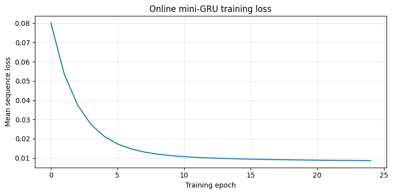
With the fixed seed, the final loss should be lower than the initial loss. The example deliberately resets both recurrent and eligibility state before each sequence; otherwise the two loss values would not describe the same initial condition.
What happened#
braintrace.compile discovers which MiniGRU parameters reach recurrent hidden state through ETP primitives. learner.etrace_grad then drives the whole sequence: it takes the per-step online gradient at each step, carries the accumulator across time, and applies the reduction — 'mean' divides by the number of steps. learner.etrace_evolve is the same drive without a loss, used by evaluate to advance hidden state and eligibility traces and return the outputs. brainstate.transform.for_loop performs the repeated epoch updates without repeatedly dispatching model calls from Python.
Next steps#
Core Concepts explains how ETP primitives select trainable pathways.
RNN Online Learning develops the rate-RNN workflow.
SNN Online Learning develops the spiking-network workflow.