

Event-driven computations with brainevent#


What is brainevent?#
brainevent is the event-driven computation package in the BrainX ecosystem. It provides event representations and connectivity operators for simulations where neural activity is sparse, such as spiking neural networks and event-based recurrent models.
The main reason to use brainevent is efficiency and clarity in sparse activity. At many time steps, only a small subset of neurons fires. Instead of treating every presynaptic neuron as active, a BinaryArray marks the neurons that actually fired, and event-aware multiplication visits the relevant rows or connections of the weight structure.
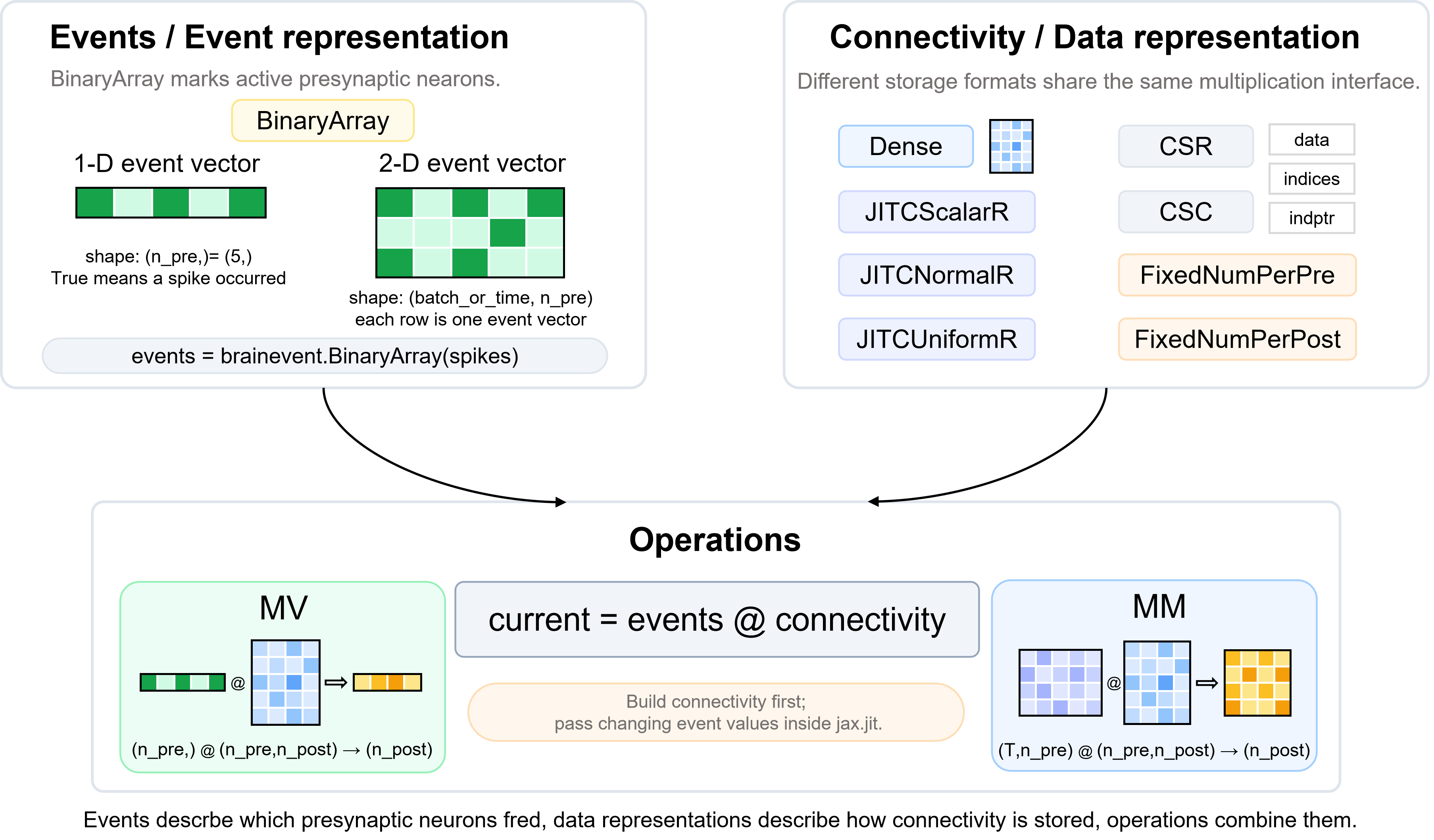
brainevent separates event-driven computation into three parts:
Event representation: neural spikes are represented as binary events. A 1-D event vector records which presynaptic neurons fired at one simulation step, and a 2-D event block records the same information across a batch or a short time window. Wrapping these arrays with
brainevent.BinaryArraytellsbraineventthat the input is sparse activity, so event-driven kernels can skip silent neurons.Data representation: the connection weights from presynaptic neurons to postsynaptic neurons can be stored in different formats. Dense matrices are simple and useful for small examples; CSR sparse matrices compactly store explicit sparse connectivity; JIT-generated connectivity represents large random graphs without materializing every edge ahead of time; and fixed fan-in or fan-out structures are useful when each neuron has a constrained number of connections.
Operations: operations combine an event representation with a data representation. The common forward projection is written as
event @ Worevents @ W: active presynaptic events select rows or connections fromW, and their weights are accumulated onto postsynaptic targets. Reverse products are also available when target-side signals need to be projected back through the same connectivity, for example in feedback, readout, or learning-signal computations.
This tutorial follows one small event vector through the main representations used in practice: dense matrices for clarity, CSR for explicit sparse connectivity, JIT-generated connectivity for large random graphs, and fixed connection-count structures for constrained fan-in or fan-out.
You will learn how to:
represent binary spike events with
brainevent.BinaryArray;read matrix-vector (
mv) and matrix-matrix (mm) event operations;build and use dense, CSR, JIT, and fixed connectivity structures;
place event-driven multiplication inside a
jax.jitfunction without rebuilding connectivity inside the compiled function.
For deeper explanations, extended examples, and complete API references, read the full brainevent documentation.
1. Imports#
The examples use small arrays so that the structure is easy to inspect. In a real simulation, the same APIs are intended for sparse, large-scale event streams.
import brainevent
import jax
import jax.numpy as jnp
import numpy as np
2. Binary events#
A spike train at one time step is naturally represented as a boolean or binary vector:
Trueor1: the neuron fired;Falseor0: the neuron was silent.
brainevent.BinaryArray wraps this event vector and tells downstream operators to use event-driven kernels where possible. The object exposes array-like metadata such as shape and dtype, supports indexing, and stores the raw JAX array in .value for ordinary reductions or inspection.
# Five presynaptic neurons at one simulation step.
spikes_bool = jnp.array([True, False, True, False, True])
events = brainevent.BinaryArray(spikes_bool)

print("Binary event representation")
print(f"  events      = {events}")
print(f"  raw values  = {events.value}")
print(f"  shape       = {events.shape}")
print(f"  spike count = {events.value.sum()}")
print(f"  active ids  = {jnp.where(events.value)[0]}")
Binary event representation
  events      = BinaryArray(value=[ True False  True False  True], dtype=bool)
  raw values  = [ True False  True False  True]
  shape       = (5,)
  spike count = 3
  active ids  = [0 2 4]
A two-dimensional BinaryArray represents a batch or a short time block. In this case, matrix multiplication becomes an mm operation: a binary event matrix times a weight matrix.
# Three time steps, five neurons.
event_block = brainevent.BinaryArray(jnp.array([
    [True,  False, True,  False, False],
    [False, True,  False, False, True ],
    [True,  True,  False, True,  False],
]))

print("Binary event block")
print(f"  shape = {event_block.shape}")
print(f"  spike counts per step = {event_block.value.sum(axis=1)}")
Binary event block
  shape = (3, 5)
  spike counts per step = [2 2 3]
3. Operation semantics: mv and mm#
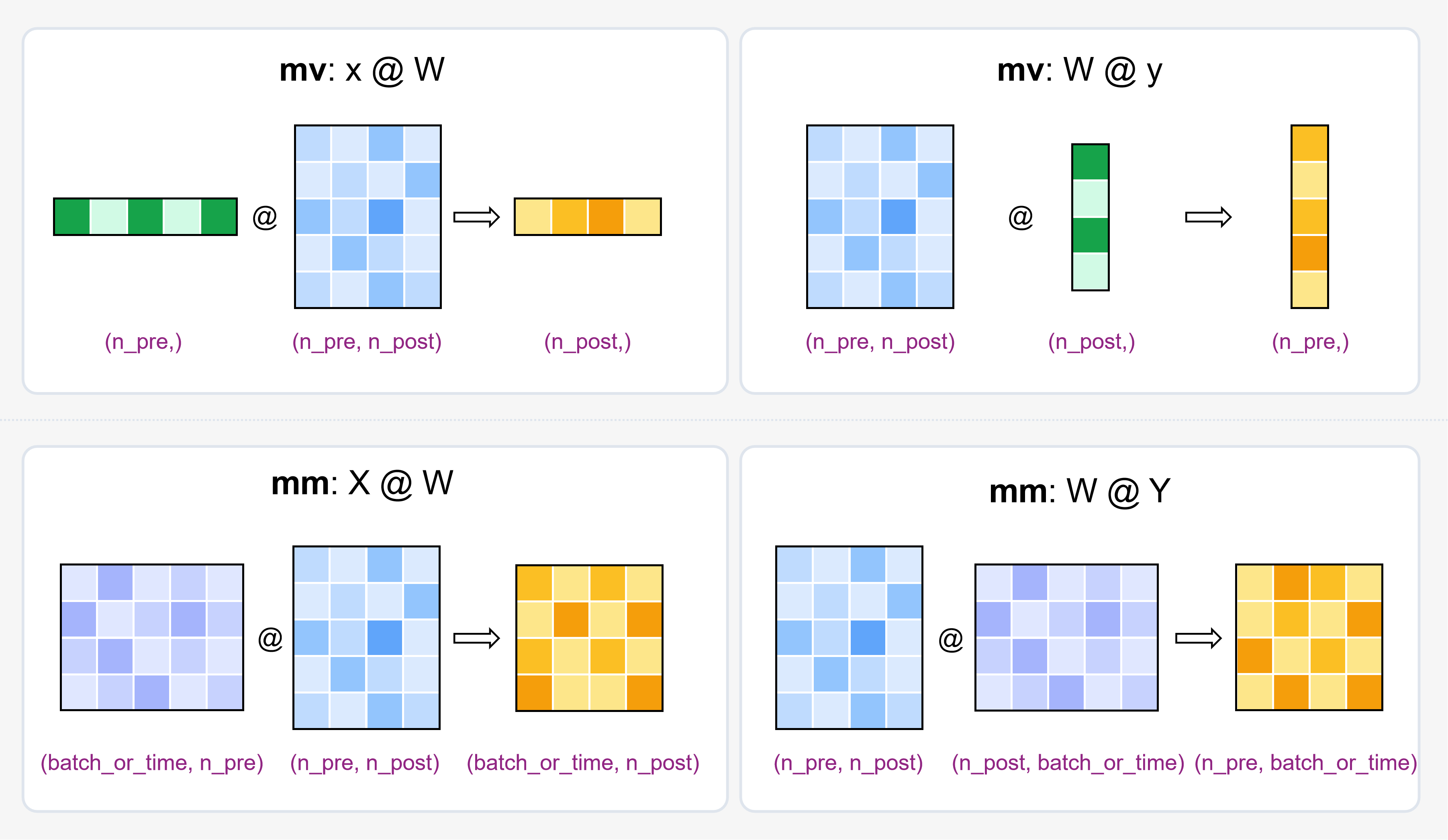
brainevent keeps the same algebra as ordinary matrix multiplication. The forward convention in this tutorial is x @ W: x is a presynaptic event vector or event block, and W has shape (n_pre, n_post). The implementation may call a transposed low-level kernel internally so that the event axis becomes the axis visited by the event-driven kernel. This lets the kernel skip inactive events while preserving the same user-facing @ algebra as the dense reference.
Expression |
Event input |
Connectivity |
Name |
Result |
|---|---|---|---|---|
|
|
|
|
|
|
|
|
|
|
The opposite side is also supported when the event shape matches the postsynaptic axis: W @ y with y.shape == (n_post,) returns (n_pre,), and W @ Y with Y.shape == (n_post, batch_or_time) returns (n_pre, batch_or_time). Physically, W @ Y is a target-to-source aggregation: Y marks active postsynaptic, target-side events or gates, and the product accumulates their weighted influence back onto each presynaptic source neuron. This can be useful for feedback, readout or credit signals, and algorithms that project postsynaptic activity back through the same connectivity. It is a different algebraic product from forward propagation, not a replacement for x @ W.
Common pitfalls:
Store weights as
(n_pre, n_post): rows are presynaptic sources, columns are postsynaptic targets.Treat the leading dimension of a 2-D left-hand
BinaryArrayas batch or time, not as another neuron axis.Build
CSR, fixed, and JIT connectivity objects before enteringjax.jit. Inside a compiled function, pass the changing spike values, wrap them withBinaryArray, and multiply by the prebuilt connectivity object.
The following sections reuse this convention for every connectivity representation.
4. Dense or general matrix data#
Dense JAX arrays are the easiest way to start because they make the expected result transparent. If x is a BinaryArray and W is a dense matrix, x @ W computes postsynaptic input by summing the rows whose presynaptic events are active.
Use dense matrices for teaching, debugging, and small examples. The sparse and structured representations below keep the same multiplication syntax while changing how the connectivity is stored or generated.
# Dense weights: 5 presynaptic neurons -> 3 postsynaptic neurons.
dense_w = jnp.array([
    [0.8, 0.0, 0.2],
    [0.1, 0.7, 0.0],
    [0.4, 0.3, 0.9],
    [0.0, 0.5, 0.6],
    [0.2, 0.0, 0.5],
], dtype=jnp.float32)

# Matrix-vector: one event vector times one weight matrix.
dense_mv = events @ dense_w

# Matrix-matrix: a block of event vectors times the same weight matrix.
dense_mm = event_block @ dense_w

print("Dense/general matrix operations")
print(f"  dense_w shape = {dense_w.shape}")
print(f"  mv result     = {dense_mv}")
print(f"  mm shape      = {dense_mm.shape}")
print(dense_mm)
Dense/general matrix operations
  dense_w shape = (5, 3)
  mv result     = [1.4000001 0.3       1.6      ]
  mm shape      = (3, 3)
[[1.2        0.3        1.1       ]
 [0.3        0.7        0.5       ]
 [0.90000004 1.2        0.8       ]]
The @ operator is the recommended high-level interface throughout this tutorial. It lets the same event code work with dense arrays, CSR matrices, fixed structures, and JIT connectivity. Lower-level kernels are useful when implementing custom operators or benchmarking internals, but they are not needed for ordinary tutorial code.
# The event-driven result matches ordinary dense multiplication.
reference_mv = events.value.astype(dense_w.dtype) @ dense_w
reference_mm = event_block.value.astype(dense_w.dtype) @ dense_w

print("Dense reference check")
print(f"  mv matches dense reference: {jnp.allclose(dense_mv, reference_mv)}")
print(f"  mm matches dense reference: {jnp.allclose(dense_mm, reference_mm)}")
Dense reference check
  mv matches dense reference: True
  mm matches dense reference: True
5. CSR sparse connectivity#
Real neural connectivity is usually sparse. CSR, compressed sparse row, stores a matrix row by row:
data: non-zero weights;indices: column index for each stored weight;indptr: offsets showing where each row starts and ends indataandindices.
CSR is a natural format for forward event propagation because each active presynaptic neuron selects a row, and only the non-zero outgoing connections in that row are visited.
# Build the same 5 -> 3 matrix from coordinate triplets.
row = jnp.array([0, 0, 1, 1, 2, 2, 2, 3, 3, 4, 4])
col = jnp.array([0, 2, 0, 1, 0, 1, 2, 1, 2, 0, 2])
data = jnp.array([0.8, 0.2, 0.1, 0.7, 0.4, 0.3, 0.9, 0.5, 0.6, 0.2, 0.5], dtype=jnp.float32)

indptr, indices, order = brainevent.coo2csr(row, col, shape=(5, 3))
csr_w = brainevent.CSR((data[order], indices, indptr), shape=(5, 3))

print("CSR representation")
print(f"  shape   = {csr_w.shape}")
print(f"  nse     = {csr_w.nse}")
print(f"  data    = {csr_w.data}")
print(f"  indices = {csr_w.indices}")
print(f"  indptr  = {csr_w.indptr}")
print("Dense view:")
print(csr_w.todense())
CSR representation
  shape   = (5, 3)
  nse     = 11
  data    = [0.8 0.2 0.1 0.7 0.4 0.3 0.9 0.5 0.6 0.2 0.5]
  indices = [0 2 0 1 0 1 2 1 2 0 2]
  indptr  = [ 0  2  4  7  9 11]
Dense view:
[[0.8 0.  0.2]
 [0.1 0.7 0. ]
 [0.4 0.3 0.9]
 [0.  0.5 0.6]
 [0.2 0.  0.5]]
csr_mv = events @ csr_w
csr_mm = event_block @ csr_w

print("CSR event-driven operations")
print(f"  mv result = {csr_mv}")
print(f"  mm shape  = {csr_mm.shape}")
print(csr_mm)
print()
print("Consistency with dense weights")
print(f"  mv matches: {jnp.allclose(csr_mv, dense_mv)}")
print(f"  mm matches: {jnp.allclose(csr_mm, dense_mm)}")
CSR event-driven operations
  mv result = [1.4000001 0.3       1.6      ]
  mm shape  = (3, 3)
[[1.2        0.3        1.1       ]
 [0.3        0.7        0.5       ]
 [0.90000004 1.2        0.8       ]]

Consistency with dense weights
  mv matches: True
  mm matches: True
CSR is usually the first sparse structure to reach for when the connection graph is known and sparse. It keeps the graph explicit, is easy to compare against a dense reference, and works with the same events @ weights syntax used above.
6. CSC and orientation#
CSC, compressed sparse column, stores the same idea column by column. It is useful when algorithms need efficient access by postsynaptic target or column. The forward examples below use CSR because a presynaptic event vector naturally activates rows, but it is useful to recognize both formats in API references and conversion utilities.
# A CSC object can store the same dense matrix by columns.
# Column 0: rows 0, 1, 2, 4
# Column 1: rows 1, 2, 3
# Column 2: rows 0, 2, 3, 4
csc_data = jnp.array([0.8, 0.1, 0.4, 0.2, 0.7, 0.3, 0.5, 0.2, 0.9, 0.6, 0.5], dtype=jnp.float32)
csc_indices = jnp.array([0, 1, 2, 4, 1, 2, 3, 0, 2, 3, 4])
csc_indptr = jnp.array([0, 4, 7, 11])
csc_w = brainevent.CSC((csc_data, csc_indices, csc_indptr), shape=(5, 3))

print("CSC representation")
print(f"  shape   = {csc_w.shape}")
print(f"  nse     = {csc_w.nse}")
print("Dense view:")
print(csc_w.todense())
CSC representation
  shape   = (5, 3)
  nse     = 11
Dense view:
[[0.8 0.  0.2]
 [0.1 0.7 0. ]
 [0.4 0.3 0.9]
 [0.  0.5 0.6]
 [0.2 0.  0.5]]
7. JIT dynamic connectivity#
Sometimes storing the full connection matrix is still too expensive. JIT connectivity structures store the random rule, not every sampled edge. During multiplication, the operator regenerates the needed random connections from the rule and seed.
Useful JIT connectivity families include:
JITCScalarR: Bernoulli connections with one scalar weight;JITCNormalR: Bernoulli connections with weights sampled from a normal distribution;JITCUniformR: Bernoulli connections with weights sampled from a uniform distribution.
The R suffix means row-oriented, which is usually the right orientation for forward propagation from presynaptic events.
# Homogeneous random connections: (weight, probability, seed).
jit_w = brainevent.JITCScalarR(
    (0.2, 0.4, 2024),
    shape=(5, 3),
)

jit_mv = events @ jit_w
jit_mm = event_block @ jit_w

print("JIT dynamic connectivity")
print(f"  shape = {jit_w.shape}")
print(f"  weight = {jit_w.weight}")
print(f"  probability = {jit_w.prob}")
print(f"  seed = {jit_w.seed}")
print(f"  mv result = {jit_mv}")
print(f"  mm result shape = {jit_mm.shape}")
print(jit_mm)
JIT dynamic connectivity
  shape = (5, 3)
  weight = 0.20000000298023224
  probability = 0.4
  seed = 2024
  mv result = [0.4 0.  0. ]
  mm result shape = (3, 3)
[[0.2 0.  0. ]
 [0.2 0.2 0.2]
 [0.2 0.2 0.2]]
# Distribution-based JIT connectivity uses the same multiplication pattern.
jit_normal = brainevent.JITCNormalR(
    (0.0, 0.1, 0.3, 7),  # (mean, std, probability, seed)
    shape=(5, 3),
)

jit_uniform = brainevent.JITCUniformR(
    (-0.1, 0.3, 0.3, 8),  # (low, high, probability, seed)
    shape=(5, 3),
)

print("Other JIT connectivity rules")
print(f"  normal mv = {events @ jit_normal}")
print(f"  uniform mv = {events @ jit_uniform}")
Other JIT connectivity rules
  normal mv = [0.25821236 0.         0.        ]
  uniform mv = [-0.09996567  0.         -0.06874797]
JIT connectivity uses the same multiplication pattern as dense and CSR connectivity. Keep the rule object outside performance-critical loops, then reuse it with changing event values. This keeps tutorial code close to the way a larger simulation would be written.
8. Fixed connection-count structures#
Fixed connectivity structures are useful when each neuron should have a fixed number of partners.
FixedNumPerPre: each presynaptic neuron stores a fixed number of postsynaptic targets. This is a fixed fan-out representation.FixedNumPerPost: each postsynaptic neuron stores a fixed number of presynaptic sources. This is a fixed fan-in representation.
Both store two compact arrays: weights and integer indices. These names are the current brainevent API in version 0.1.0.
# Fixed fan-out: each presynaptic neuron connects to two postsynaptic neurons.
fixed_pre_indices = jnp.array([
    [0, 2],
    [1, 2],
    [0, 1],
    [1, 2],
    [0, 2],
], dtype=jnp.int32)
fixed_pre_weights = jnp.array([
    [0.8, 0.2],
    [0.7, 0.1],
    [0.4, 0.3],
    [0.5, 0.6],
    [0.2, 0.5],
], dtype=jnp.float32)

fixed_pre_w = brainevent.FixedNumPerPre(
    (fixed_pre_weights, fixed_pre_indices),
    shape=(5, 3),
)

fixed_pre_mv = events @ fixed_pre_w
fixed_pre_mm = event_block @ fixed_pre_w

print("FixedNumPerPre: fixed fan-out from each presynaptic neuron")
print(f"  shape = {fixed_pre_w.shape}")
print(f"  data shape = {fixed_pre_w.data.shape}")
print(f"  indices shape = {fixed_pre_w.indices.shape}")
print("  dense view:")
print(fixed_pre_w.todense())
print(f"  mv result = {fixed_pre_mv}")
print(f"  mm result shape = {fixed_pre_mm.shape}")
FixedNumPerPre: fixed fan-out from each presynaptic neuron
  shape = (5, 3)
  data shape = (5, 2)
  indices shape = (5, 2)
  dense view:
[[0.8 0.  0.2]
 [0.  0.7 0.1]
 [0.4 0.3 0. ]
 [0.  0.5 0.6]
 [0.2 0.  0.5]]
  mv result = [1.4000001 0.3       0.7      ]
  mm result shape = (3, 3)
# Fixed fan-in: each postsynaptic neuron receives from two presynaptic neurons.
fixed_post_indices = jnp.array([
    [0, 2],
    [1, 3],
    [2, 4],
], dtype=jnp.int32)
fixed_post_weights = jnp.array([
    [0.8, 0.4],
    [0.7, 0.5],
    [0.9, 0.5],
], dtype=jnp.float32)

fixed_post_w = brainevent.FixedNumPerPost(
    (fixed_post_weights, fixed_post_indices),
    shape=(5, 3),
)

print("FixedNumPerPost: fixed fan-in to each postsynaptic neuron")
print(f"  shape = {fixed_post_w.shape}")
print(f"  data shape = {fixed_post_w.data.shape}")
print(f"  indices shape = {fixed_post_w.indices.shape}")
print("  dense view:")
print(fixed_post_w.todense())
print(f"  mv result = {events @ fixed_post_w}")
FixedNumPerPost: fixed fan-in to each postsynaptic neuron
  shape = (5, 3)
  data shape = (3, 2)
  indices shape = (3, 2)
  dense view:
[[0.8 0.  0. ]
 [0.  0.7 0. ]
 [0.4 0.  0.9]
 [0.  0.5 0. ]
 [0.  0.  0.5]]
  mv result = [1.2 0.  1.4]
Fixed fan-out and fixed fan-in structures are both multiplied with the same @ syntax. Choose the orientation that matches the model constraint you care about: fixed outgoing degree from each presynaptic neuron, or fixed incoming degree to each postsynaptic neuron.
9. JIT compilation#
brainevent is designed for JAX workflows. The usual pattern is to construct connectivity once, then compile a function that receives changing spike values.
Avoid rebuilding CSR, fixed, or JIT connectivity objects inside the compiled function. Those objects describe the graph; the spike vector is the dynamic input that changes each step.
@jax.jit
def forward_one_step(spike_values):
    spike_events = brainevent.BinaryArray(spike_values)
    return spike_events @ csr_w

compiled_output = forward_one_step(spikes_bool)
print("JIT-compiled one-step forward pass")
print(compiled_output)
JIT-compiled one-step forward pass
[1.4000001 0.3       1.6      ]
10. Choosing a representation#
Representation |
What it stores |
Best for |
Typical operation |
|---|---|---|---|
Dense/general matrix |
every weight |
small examples, debugging, dense layers |
|
|
non-zero weights by presynaptic row |
known sparse forward connectivity |
|
|
non-zero weights by postsynaptic column |
column-oriented algorithms and conversions |
inspect or convert by target |
|
random rule and seed |
very large random networks |
|
|
fixed fan-out targets per presynaptic neuron |
biologically constrained outgoing degree |
|
|
fixed fan-in sources per postsynaptic neuron |
biologically constrained incoming degree |
|
A useful workflow is to start with dense matrices while checking the math, switch to CSR when the graph is known and sparse, use JIT connectivity when random connectivity is too large to store, and use fixed structures when degree constraints are part of the model.
11. Mini example: event-driven layer#
The final example wraps the same ideas into a small layer. It accepts binary presynaptic activity, converts it to BinaryArray, and multiplies it by whichever connectivity representation you pass in.
def event_layer(spike_values, weights, threshold=0.5):
    input_events = brainevent.BinaryArray(spike_values)
    current = input_events @ weights
    output_events = brainevent.BinaryArray(current > threshold)
    return current, output_events

for name, weights in [
    ("dense", dense_w),
    ("CSR", csr_w),
    ("FixedNumPerPre", fixed_pre_w),
    ("JITCScalarR", jit_w),
]:
    current, output_events = event_layer(spikes_bool, weights)
    print(f"{name}")
    print(f"  current = {current}")
    print(f"  output spikes = {output_events.value}")
dense
  current = [1.4000001 0.3       1.6      ]
  output spikes = [ True False  True]
CSR
  current = [1.4000001 0.3       1.6      ]
  output spikes = [ True False  True]
FixedNumPerPre
  current = [1.4000001 0.3       0.7      ]
  output spikes = [ True False  True]
JITCScalarR
  current = [0.4 0.  0. ]
  output spikes = [False False False]