State-based transformations with brainstate

What is brainstate?

brainstate is the state-management and transformation package in the BrainX ecosystem. It helps you write neural models whose variables change over time, such as membrane potentials, spike states, synaptic states, hidden states, and trainable parameters.

In ordinary JAX code, mutable model state needs careful handling because transformations such as jit, vmap, and grad expect explicit, functional data flow. brainstate provides state objects, module abstractions, environment control, and state-aware transformations so that stateful neural dynamics can still be simulated, compiled, vectorized, and differentiated in a JAX-native way.

This tutorial focuses on state-based transformations: the tools that make stateful brain simulations easier to run efficiently and correctly. You will learn:

• How to use for_loop for sequential time-step simulations

• When and how to apply jit (Just-In-Time compilation) for performance

• Using vmap for vectorization across multiple trials or batches

• Using map for memory-efficient batching

• Using cond for conditional branching in JIT-compiled code

• Using grad for automatic differentiation and optimization

• Combining transformations for complex simulation workflows

• Best practices and common patterns

For complete API details, state-management concepts, and advanced transformation examples, read the full brainstate documentation.

Setup and Imports

import braintools
import brainstate
import brainunit as u
import jax
import jax.numpy as jnp
import numpy as np
import matplotlib.pyplot as plt

# Set global simulation time step
brainstate.environ.set(dt=0.1 * u.ms)

What are Transformations?

In brainstate, transformations are function decorators and utilities that modify how your neural dynamics code executes:

1. for_loop: Sequentially iterates over time steps or data, managing state updates automatically

2. jit: Just-In-Time compiles your functions for faster execution on CPU/GPU/TPU

3. vmap: Vectorizes (batches) computations across multiple trials or parameter sets

4. map: Memory-efficient batching when full vmap would exceed memory

5. cond: Enables conditional branching in JIT-compiled code for event-driven dynamics

6. grad: Computes gradients automatically for optimization and learning

These transformations handle the complex bookkeeping of stateful computations, allowing you to write simple, readable code while achieving high performance.

Example Model: Simple LIF Neuron

Let’s define a simple LIF neuron model that we’ll use throughout this tutorial.

from typing import Callable

class LIFDynamics(brainstate.nn.Dynamics):
    """
    A leaky integrate-and-fire neuron implemented as a Dynamics module.
    This implementation matches the working example from brainstate_LIF_neuron.ipynb.
    """
    def __init__(
        self,
        in_size: brainstate.typing.Size,
        R: brainstate.typing.ArrayLike = 1.0 * u.ohm,
        tau: brainstate.typing.ArrayLike = 5.0 * u.ms,
        V_th: brainstate.typing.ArrayLike = 1.0 * u.mV,
        V_reset: brainstate.typing.ArrayLike = 0.0 * u.mV,
        V_rest: brainstate.typing.ArrayLike = 0.0 * u.mV,
        V_initializer: Callable = braintools.init.Constant(0.0 * u.mV),
        spk_fun: Callable = braintools.surrogate.ReluGrad(),
        spk_reset: str = "soft",
        name: str | None = None,
    ):
        super().__init__(in_size, name=name)
        # Parameters (unit-aware)
        self.R = braintools.init.param(R, self.varshape)
        self.tau = braintools.init.param(tau, self.varshape)
        self.V_th = braintools.init.param(V_th, self.varshape)
        self.V_reset = braintools.init.param(V_reset, self.varshape)
        self.V_rest = braintools.init.param(V_rest, self.varshape)
        self.V_initializer = V_initializer
        # Spiking
        self.spk_fun = spk_fun
        self.spk_reset = spk_reset

    def init_state(self, batch_size: int | None = None, **kwargs):
        self.V = brainstate.HiddenState(
            braintools.init.param(self.V_initializer, self.varshape, batch_size)
        )

    def reset_state(self, batch_size: int | None = None, **kwargs):
        self.V.value = braintools.init.param(self.V_initializer, self.varshape, batch_size)

    def get_spike(self, V=None):
        V = self.V.value if V is None else V
        v_scaled = (V - self.V_th) / (self.V_th - self.V_reset)
        return self.spk_fun(v_scaled)

    def update(self, x=0.0 * u.mA):
        last_v = self.V.value
        spk = self.get_spike(last_v)
        # Reset policy
        V_th_or_v = self.V_th if self.spk_reset == 'soft' else jax.lax.stop_gradient(last_v)
        V = last_v - (V_th_or_v - self.V_reset) * spk
        # Dynamics integration by exponential Euler
        dv = lambda v: (-(v - self.V_rest) + self.R * x) / self.tau
        V = brainstate.nn.exp_euler_step(dv, V)
        self.V.value = V
        return self.get_spike(V)


# Helper function to run simulations
def run_lif(lif_module, inputs, reset=True):
    """Run the LIF over a 1D array of input currents.
    
    Returns membrane potentials and spikes over time.
    """
    if reset:
        lif_module.reset_state()
    
    # Safely get the length of inputs (robust for all array types)
    inputs = u.math.asarray(inputs)  # Ensure it's an array
    n_steps = inputs.shape[0] if hasattr(inputs, 'shape') and len(inputs.shape) > 0 else 1
    idx = np.arange(n_steps)

    def step(i, x):
        with brainstate.environ.context(i=i):
            s = lif_module(x)
            return lif_module.V.value, s

    V_seq, S_seq = brainstate.transform.for_loop(step, idx, inputs)
    return V_seq, S_seq


# Create and initialize the model
neuron = LIFDynamics(in_size=1)
brainstate.nn.init_all_states(neuron)
print(neuron)

LIFDynamics(
  in_size=(1,),
  out_size=(1,),
  R=Quantity(1., "ohm"),
  tau=Quantity(5., "ms"),
  V_th=Quantity(1., "mV"),
  V_reset=Quantity(0., "mV"),
  V_rest=Quantity(0., "mV"),
  V_initializer=Constant(value=0. mV),
  spk_fun=ReluGrad(alpha=0.3, width=1.0),
  spk_reset=soft,
  V=HiddenState(
    value=Quantity(~float32[1], "mV")
  )
)

Transformation 1: for_loop

The for_loop transformation is the workhorse of sequential simulation. It:

• Iterates over time steps or input sequences

• Automatically manages state updates between iterations

• Optionally displays progress bars

• Returns collected outputs from each step

Basic Usage

The typical pattern is:

def step_function(index, *inputs):
    # Your simulation logic here
    with brainstate.environ.context(i=index):
        output = model(*inputs)
    return output

results = brainstate.transform.for_loop(step_function, indices, inputs)

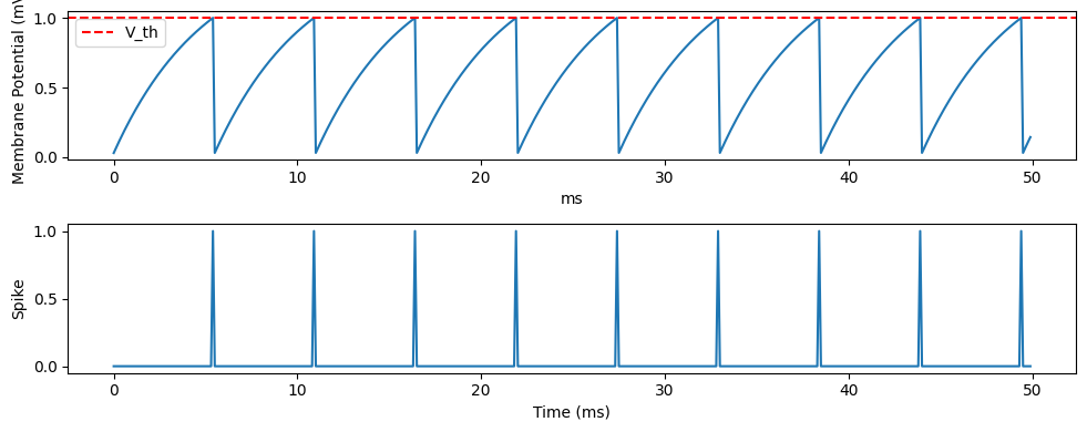
# Simulate for 500 time steps with constant input
n_steps = 500
inputs = np.ones(n_steps) * 1.5 * u.mA  # Constant input current

# Run simulation using helper function
V_trace, spike_trace = run_lif(neuron, inputs)

# Plot results
times = np.arange(n_steps) * brainstate.environ.get_dt()
plt.figure(figsize=(10, 4))
plt.subplot(2, 1, 1)
plt.plot(times, V_trace)
plt.axhline(neuron.V_th.mantissa, color='r', linestyle='--', label='V_th')
plt.ylabel('Membrane Potential (mV)')
plt.legend()
plt.subplot(2, 1, 2)
plt.plot(times, spike_trace)
plt.ylabel('Spike')
plt.xlabel('Time (ms)')
plt.tight_layout()
plt.show()

Progress Bars

For long simulations, you can add a progress bar:

# Long simulation with progress bar
n_steps = 10000
inputs = np.ones(n_steps) * 1.5 * u.mA

neuron.reset_state()
idx = np.arange(n_steps)

def step(i, x):
    with brainstate.environ.context(i=i):
        s = neuron(x)
        return neuron.V.value, s

V_trace, spike_trace = brainstate.transform.for_loop(
    step, 
    idx, 
    inputs,
    pbar=brainstate.transform.ProgressBar(1000)  # Update every 1000 steps
    # or simply
    # pbar=1000
)

print(f"Simulation completed: {n_steps} steps")

Simulation completed: 10000 steps

Transformation 2: jit (Just-In-Time Compilation)

JIT compilation can dramatically speed up your simulations by compiling Python/NumPy code to optimized machine code. Use jit when:

• You’re running long simulations

• The function will be called many times

• Performance is critical

Basic JIT Usage

You can JIT-compile simulation functions. Note that we need to be careful with how we structure the code for JIT:

# Create a separate neuron for JIT example
jit_neuron = LIFDynamics(in_size=1)
brainstate.nn.init_all_states(jit_neuron)

def run_simulation_nojit(inputs):
    """Non-JIT simulation function."""
    return run_lif(jit_neuron, inputs)

@brainstate.transform.jit
def run_simulation_jit(inputs):
    """JIT-compiled simulation function."""
    return run_lif(jit_neuron, inputs)

# Benchmark
import time
inputs = np.ones(5000) * 1.5 * u.mA

# Non-JIT
start = time.time()
V1, S1 = run_simulation_nojit(inputs)
nojit_time = time.time() - start

# First JIT call: includes compilation (slower)
start = time.time()
V2, S2 = run_simulation_jit(inputs)
compile_time = time.time() - start

# Second JIT call: uses compiled version (much faster)
start = time.time()
V3, S3 = run_simulation_jit(inputs)
run_time = time.time() - start

print(f"No JIT: {nojit_time:.4f}s")
print(f"First JIT call (with compilation): {compile_time:.4f}s")
print(f"Second JIT call (compiled): {run_time:.4f}s")
if run_time > 0:
    print(f"Speedup: {nojit_time/run_time:.1f}x")
else:
    print(f"Speedup: Very fast (>1000x)")

No JIT: 0.0390s
First JIT call (with compilation): 0.0386s
Second JIT call (compiled): 0.0010s
Speedup: 39.0x

Transformation 3: vmap (Vectorization)

vmap (vectorized map) runs your function in parallel over a batch dimension. This is incredibly useful for:

• Running multiple trials with different random seeds

• Sweeping parameters

• Processing multiple inputs simultaneously

Running Multiple Trials

Let’s run multiple trials with different input currents:

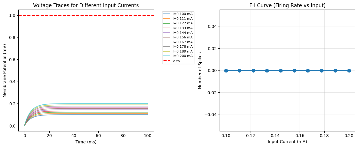
# Different input currents for each trial
batch_size = 10
n_steps = 1000
input_currents = np.linspace(0.1, 0.2, batch_size) * u.mA

# Create batched inputs: shape (batch, time)
inputs_list = []
for I in input_currents:
    inputs_list.append(np.ones(n_steps) * I)
inputs_batched = u.math.asarray(inputs_list)

# IMPORTANT: Create NEW neuron instances inside vmap to avoid state conflicts
@brainstate.transform.vmap
def run_batched_trial(inp_seq):
    """Run simulation for a single input sequence.
    
    Key Pattern: Create a fresh LIF instance for each vmap iteration.
    This avoids BatchAxisError from shared state across iterations.
    """
    lif_single = LIFDynamics(1)
    brainstate.nn.init_all_states(lif_single)
    
    # Safely get sequence length
    inp_seq = u.math.asarray(inp_seq)
    n_steps_local = inp_seq.shape[0] if hasattr(inp_seq, 'shape') and len(inp_seq.shape) > 0 else 1
    idx = np.arange(n_steps_local)

    def step(i, x):
        with brainstate.environ.context(i=i):
            s = lif_single(x)
            return lif_single.V.value, s
    
    return brainstate.transform.for_loop(step, idx, inp_seq)

# Run all trials in parallel
V_batch, S_batch = run_batched_trial(inputs_batched)

print(f"Output shape: V_batch={V_batch.shape}, S_batch={S_batch.shape}")
print(f"Expected: (batch={batch_size}, time={n_steps}, neurons=1)")

Output shape: V_batch=(10, 1000, 1), S_batch=(10, 1000, 1)
Expected: (batch=10, time=1000, neurons=1)

Visualizing Batch Results

# Plot membrane potentials for all trials
times = np.arange(n_steps) * brainstate.environ.get_dt()
plt.figure(figsize=(12, 5))

plt.subplot(1, 2, 1)
for i in range(batch_size):
    plt.plot(times, V_batch[i, :, 0].mantissa, alpha=0.7,
             label=f'I={input_currents[i].mantissa:.3f} mA')
plt.axhline(1.0, color='r', linestyle='--', linewidth=2, label='V_th')
plt.xlabel('Time (ms)')
plt.ylabel('Membrane Potential (mV)')
plt.title('Voltage Traces for Different Input Currents')
plt.legend(bbox_to_anchor=(1.05, 1), loc='upper left', fontsize=8)

plt.subplot(1, 2, 2)
# Count spikes for each trial (threshold at 0.5)
spike_counts = []
for i in range(batch_size):
    count = (np.asarray(S_batch[i]) >= 0.5).sum()
    spike_counts.append(count)

plt.plot(input_currents.mantissa, spike_counts, 'o-', markersize=8, linewidth=2)
plt.xlabel('Input Current (mA)')
plt.ylabel('Number of Spikes')
plt.title('F-I Curve (Firing Rate vs Input)')
plt.grid(True, alpha=0.3)

plt.tight_layout()
plt.show()

Combining Transformations

The real power comes from combining transformations. A common pattern is jit + vmap for fast, batched simulations:

# Combined JIT + vmap for maximum performance
import time

n_trials = 50
n_steps = 2000

# Create test inputs: same current for all trials
test_inputs_list = []
for _ in range(n_trials):
    test_inputs_list.append(np.ones(n_steps) * 1.5 * u.mA)
test_inputs = u.math.asarray(test_inputs_list)

@brainstate.transform.jit
@brainstate.transform.vmap
def fast_batch_simulation(inp_seq):
    """JIT-compiled, vectorized simulation.
    
    Creates a fresh neuron for each vmap iteration (best practice).
    """
    lif_fast = LIFDynamics(1)
    brainstate.nn.init_all_states(lif_fast)
    
    # Safely get sequence length
    inp_seq = u.math.asarray(inp_seq)
    n_steps_local = inp_seq.shape[0] if hasattr(inp_seq, 'shape') and len(inp_seq.shape) > 0 else 1
    idx = np.arange(n_steps_local)

    def step(i, x):
        with brainstate.environ.context(i=i):
            s = lif_fast(x)
            return lif_fast.V.value, s
    
    return brainstate.transform.for_loop(step, idx, inp_seq)

# Warm-up compilation
_ = fast_batch_simulation(test_inputs)

# Timed run
start = time.time()
V_fast, S_fast = fast_batch_simulation(test_inputs)
elapsed = time.time() - start

print(f"Ran {n_trials} trials of {n_steps} steps in {elapsed:.4f}s")
print(f"Average time per trial: {elapsed/n_trials*1000:.2f}ms")
print(f"Time per step per trial: {elapsed/(n_trials*n_steps)*1e6:.2f}µs")

Ran 50 trials of 2000 steps in 0.0000s
Average time per trial: 0.00ms
Time per step per trial: 0.00µs

Transformation 4: map for Memory-Efficient Batching

When you have many trials but limited memory, use map instead of vmap. It processes data in smaller batches sequentially:

# Simulate a scenario with many trials
n_trials_map = 100
n_steps_map = 1000

# Create inputs for all trials
large_inputs_list = []
for _ in range(n_trials_map):
    large_inputs_list.append(np.ones(n_steps_map) * 1.5 * u.mA)
large_inputs = u.math.asarray(large_inputs_list)

@brainstate.transform.vmap
def single_trial_sim(inp_seq):
    """Single trial simulation - creates its own neuron instance."""
    lif_trial = LIFDynamics(1)
    brainstate.nn.init_all_states(lif_trial)
    
    # Safely get sequence length
    inp_seq = u.math.asarray(inp_seq)
    n_steps_local = inp_seq.shape[0] if hasattr(inp_seq, 'shape') and len(inp_seq.shape) > 0 else 1
    idx = np.arange(n_steps_local)

    def step(i, x):
        with brainstate.environ.context(i=i):
            return lif_trial(x)
    
    return brainstate.transform.for_loop(step, idx, inp_seq)

spike_results = single_trial_sim(large_inputs)
print(f"Processed {n_trials_map} trials")
print(f"Output shape: {spike_results.shape}")

total_spikes = 0
for i in range(n_trials_map):
    spike_trace = spike_results[i]
    if hasattr(spike_trace, '__len__'):
        total_spikes += (np.asarray(spike_trace) >= 0.5).sum()
print(f"Total spikes across all trials: {total_spikes}")

Processed 100 trials
Output shape: (100, 1000, 1)
Total spikes across all trials: 1800

Advanced Pattern: Nested Loops

Sometimes you need nested iteration (e.g., trials × time steps). Here’s a practical example with random noise:

nested_neuron = LIFDynamics(1)
brainstate.nn.init_all_states(nested_neuron)

n_trials_nest = 5
n_steps_nest = 500

def run_single_trial_noise(trial_idx):
    """Run one trial with a specific random seed."""
    nested_neuron.reset_state()
    
    # Generate noisy input for this trial
    key = jax.random.PRNGKey(trial_idx)
    base_current = 1.5 * u.mA
    noise = jax.random.normal(key, (n_steps_nest,)) * 0.03 * u.mA
    inputs = base_current + noise
    
    # Run simulation and return spike count
    _, spikes = run_lif(nested_neuron, inputs, reset=False)
    # return (np.asarray(spikes) >= 0.5).sum()
    spike_mask = spikes >= 0.5
    spike_count = spike_mask.sum()
    return spike_count

# Outer loop: iterate over trials
trial_indices = jnp.arange(n_trials_nest)
spike_counts = brainstate.transform.for_loop(
    lambda i: run_single_trial_noise(i), 
    trial_indices
)

print(f"Spike counts per trial: {spike_counts}")
print(f"Mean: {spike_counts.mean():.1f}, Std: {spike_counts.std():.2f}")

Spike counts per trial: [9 9 9 9 9]
Mean: 9.0, Std: 0.00

Transformation 5: cond for Conditional Branching

The cond transformation enables efficient conditional execution in JIT-compiled code. Unlike Python’s if/else, which are resolved at trace time, cond supports runtime conditionals that work seamlessly with JIT compilation.

Use cond when:

• You need data-dependent branching inside JIT-compiled functions

• Implementing different update rules based on runtime conditions

• Switching between computational modes (e.g., training vs inference)

Basic Usage

The basic pattern is:

result = brainstate.transform.cond(
    predicate,      # Boolean condition
    true_fun,       # Function called if True  
    false_fun,      # Function called if False
    operand         # Passed to whichever function is called
)

Both true_fun and false_fun must accept the same input and return the same output type/shape.

# Simple example: Apply different scaling factors based on a threshold
def adaptive_scale(x, threshold):
    """Apply 2x scaling if x > threshold, otherwise apply 0.5x scaling."""
    
    def high_branch(val):
        return val * 2.0
    
    def low_branch(val):
        return val * 0.5
    
    return brainstate.transform.cond(
        x > threshold,
        high_branch,
        low_branch,
        x
    )

# Test with different values
test_vals = jnp.array([0.5, 1.0, 1.5, 2.0, 2.5])
threshold = 1.5

print("Input | Condition | Output")
print("------|-----------|-------")
for val in test_vals:
    result = adaptive_scale(val, threshold)
    cond_str = "high" if val > threshold else "low"
    print(f"{val:.1f}   | {cond_str:9s} | {result:.1f}")

Input | Condition | Output
------|-----------|-------
0.5   | low       | 0.2
1.0   | low       | 0.5
1.5   | low       | 0.8
2.0   | high      | 4.0
2.5   | high      | 5.0

Using cond in Simulations

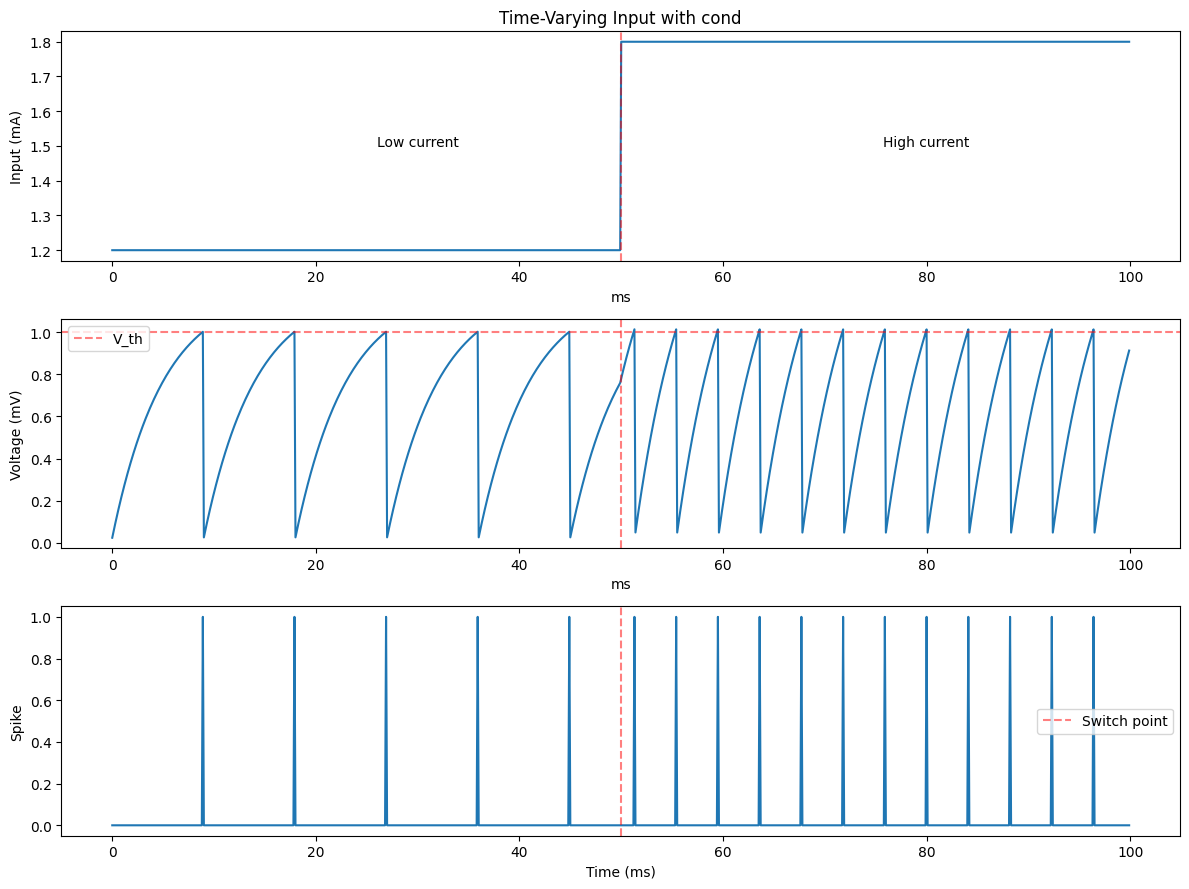
A practical use case: applying different input currents to a neuron based on time:

# Simulate neuron with time-varying input using cond
cond_neuron = LIFDynamics(1)
brainstate.nn.init_all_states(cond_neuron)

n_steps_cond = 1000
switch_time = 500  # Switch input current at this step

def get_input_current(step_idx):
    """Return different input currents before/after switch_time."""
    
    def early_phase(_):
        return 1.2 * u.mA  # Lower current
    
    def late_phase(_):
        return 1.8 * u.mA  # Higher current
    
    return brainstate.transform.cond(
        step_idx < switch_time,
        early_phase,
        late_phase,
        None  # Operand (not used here)
    )

# Run simulation
cond_neuron.reset_state()
idx_cond = np.arange(n_steps_cond)

def step_with_cond(i, _):
    with brainstate.environ.context(i=i):
        current = get_input_current(i)
        spike = cond_neuron(current)
        return current, cond_neuron.V.value, spike

currents, V_cond, spikes_cond = brainstate.transform.for_loop(
    step_with_cond, idx_cond, jnp.zeros(n_steps_cond)
)

# Plot results
times_cond = np.arange(n_steps_cond) * brainstate.environ.get_dt()

fig, axes = plt.subplots(3, 1, figsize=(12, 9))
plt.subplots_adjust(left=0.08, right=0.98, top=0.95, bottom=0.05)

# Input current
axes[0].plot(times_cond, currents.mantissa,linewidth=1.5)
axes[0].axvline(switch_time * 0.1, color='r', linestyle='--', alpha=0.5)
axes[0].set_ylabel('Input (mA)')
axes[0].set_title('Time-Varying Input with cond')
axes[0].text(30, 1.5, 'Low current', ha='center')
axes[0].text(80, 1.5, 'High current', ha='center')

# Voltage
axes[1].plot(times_cond, V_cond[:, 0].mantissa)
axes[1].axhline(1.0, color='r', linestyle='--', alpha=0.5, label='V_th')
axes[1].axvline(switch_time * 0.1, color='r', linestyle='--', alpha=0.5)
axes[1].set_ylabel('Voltage (mV)')
axes[1].legend()

# Spikes
axes[2].plot(times_cond, spikes_cond[:, 0])
axes[2].axvline(switch_time * 0.1, color='r', linestyle='--', alpha=0.5, label='Switch point')
axes[2].set_ylabel('Spike')
axes[2].set_xlabel('Time (ms)')
axes[2].legend()

plt.tight_layout()
plt.show()

# Count spikes in each phase
early_spikes = (spikes_cond[:switch_time] >= 0.5).sum()
late_spikes = (spikes_cond[switch_time:] >= 0.5).sum()
print(f"Spikes in early phase (low current): {early_spikes}")
print(f"Spikes in late phase (high current): {late_spikes}")

Spikes in early phase (low current): 5
Spikes in late phase (high current): 12

Transformation 6: grad for Automatic Differentiation

The grad transformation computes gradients automatically, enabling optimization and learning in neural models. It supports differentiation with respect to:

• Function arguments (standard autodiff)

• Model parameters (ParamState objects)

• Combinations of both

Basic Usage

The basic pattern is:

grad_fn = brainstate.transform.grad(
    fun,                  # Function to differentiate
    argnums=None,         # Which arguments to differentiate (int or list)
    grad_states=None,     # Which State objects to differentiate
    has_aux=False,        # Whether function returns (loss, aux_data)
    return_value=False    # Whether to return loss value with gradients
)

# Example 1: Computing gradients w.r.t. function arguments

def quadratic_loss(x, y):
    """Simple quadratic loss function."""
    return jnp.sum((x - y) ** 2)

# Gradient w.r.t. first argument (x)
grad_fn_x = brainstate.transform.grad(quadratic_loss, argnums=0)

x = jnp.array([1.0, 2.0, 3.0])
y = jnp.array([0.5, 1.5, 2.5])

grad_x = grad_fn_x(x, y)
print(f"Input x: {x}")
print(f"Target y: {y}")
print(f"Gradient ∂L/∂x: {grad_x}")
print(f"Loss: {quadratic_loss(x, y):.4f}")

Input x: [1. 2. 3.]
Target y: [0.5 1.5 2.5]
Gradient ∂L/∂x: [1. 1. 1.]
Loss: 0.7500

# Gradient w.r.t. multiple arguments
grad_fn_both = brainstate.transform.grad(quadratic_loss, argnums=[0, 1])
grad_x, grad_y = grad_fn_both(x, y)
print(f"\nGradients w.r.t. both arguments:")
print(f"∂L/∂x: {grad_x}")
print(f"∂L/∂y: {grad_y}")

Gradients w.r.t. both arguments:
∂L/∂x: [1. 1. 1.]
∂L/∂y: [-1. -1. -1.]

Computing Gradients w.r.t. Model Parameters

To train neural models, we need to differentiate with respect to ParamState objects. BrainState extends JAX’s autodiff to handle stateful parameters seamlessly:

# Example 2: Training a simple linear model

class LinearRegressor(brainstate.nn.Module):
    """Simple linear regression model: y = wx + b"""

    def __init__(self, in_features: int):
        super().__init__()
        # Initialize parameters with small random values
        key = jax.random.PRNGKey(0)
        self.weight = brainstate.ParamState(jax.random.normal(key, (in_features, 1)) * 0.1)
        self.bias = brainstate.ParamState(jnp.zeros((1,)))

    def __call__(self, x):
        return jnp.dot(x, self.weight.value) + self.bias.value

# Create model and training data
model = LinearRegressor(in_features=1)

# Generate synthetic data: y = 2x + 1 + noise
# Normalize input to [0, 1] for stability
key = jax.random.PRNGKey(42)
x_train = jax.random.uniform(key, (20, 1))  # Range [0, 1]
y_train = 2.0 * x_train + 1.0 + jax.random.normal(key, (20, 1)) * 0.1

# Define loss function
def compute_loss(x_data, y_data):
    """MSE loss for the model."""
    predictions = model(x_data)
    return jnp.mean((predictions - y_data) ** 2)

# Create gradient function w.r.t. all ParamState in model
# Gradients are returned as a list in the same order as grad_states
grad_fn = brainstate.transform.grad(
    compute_loss,
    grad_states=[model.weight, model.bias],  # Explicit list order
    return_value=True
)

# Training loop 
learning_rate = 0.1  
n_epochs = 150

print(f"Initial: weight={model.weight.value[0, 0]:.4f}, bias={model.bias.value[0]:.4f}")

for epoch in range(n_epochs):
    # Compute gradients - returns tuple (grads_list, loss)
    grads, loss = grad_fn(x_train, y_train)
    
    # Unpack gradients list: [grad_weight, grad_bias]
    grad_w, grad_b = grads
    
    # Update parameters
    model.weight.value = model.weight.value - learning_rate * grad_w
    model.bias.value = model.bias.value - learning_rate * grad_b
    
    if epoch % 20 == 0:
        print(f"Epoch {epoch:3d}: loss={loss:.6f}, "
              f"weight={model.weight.value[0, 0]:.4f}, "
              f"bias={model.bias.value[0]:.4f}")

print(f"\nFinal: weight={model.weight.value[0, 0]:.4f}, bias={model.bias.value[0]:.4f}")
print(f"True parameters: weight=2.0000, bias=1.0000")

Initial: weight=0.1623, bias=0.0000
Epoch   0: loss=4.882305, weight=0.4485, bias=0.4302
Epoch  20: loss=0.053904, weight=1.3369, bias=1.4566
Epoch  40: loss=0.039217, weight=1.4816, bias=1.3671
Epoch  60: loss=0.028541, weight=1.6041, bias=1.2893
Epoch  80: loss=0.020774, weight=1.7085, bias=1.2229
Epoch 100: loss=0.015124, weight=1.7976, bias=1.1663
Epoch 120: loss=0.011013, weight=1.8736, bias=1.1180
Epoch 140: loss=0.008023, weight=1.9384, bias=1.0768

Final: weight=1.9644, bias=1.0603
True parameters: weight=2.0000, bias=1.0000

Summary

You’ve learned the core transformations in brainstate:

Transformation	Purpose	When to Use
for_loop	Sequential iteration with state	Time-step simulations, sequential data
jit	Compile to fast machine code	Long/repeated simulations, performance critical
vmap	Vectorize over batch dimension	Multiple trials, parameter sweeps, batching
map	Memory-efficient batching	Large number of trials, limited memory
cond	Conditional branching in JIT code	Event-driven dynamics, mode switching, adaptive behavior
grad	Automatic differentiation	Training networks, optimizing parameters, learning rules

For more detailed information about brainstate transformations and advanced features, please visit:

BrainState Documentation