Simulating Jansen–Rit population dynamics with brainmass

What is brainmass?

brainmass is the neural mass and whole-brain modeling package in the BrainX ecosystem. It provides population-level dynamical models, coupling mechanisms, noise processes, and simulation utilities for studying mesoscopic brain activity without modeling every neuron and spike explicitly.

Use brainmass when you want to simulate cortical population dynamics, explore how model parameters change rhythmic activity, build network-level brain simulations, or compare simulated activity with macroscopic signals such as EEG, MEG, or BOLD. The package works with brainstate for stateful simulation control and brainunit for explicit physical units, so model equations remain readable and unit-aware.

For complete model documentation, API details, and additional examples, read the full brainmass documentation.

In this tutorial, we simulate a single Jansen–Rit (JR) neural mass model node under a variety of inputs to illustrate different regimes: baseline alpha-like rhythms, sinusoidal entrainment, spike–wave-like activity, reduced inhibition, and irregular/noisy dynamics.

The JR model captures mesoscopic cortical column activity using three interacting subpopulations:

• Excitatory pyramidal cells (P) — principal output population;

• Excitatory interneurons (E) — provide excitatory feedback to P;

• Inhibitory interneurons (I) — provide inhibitory feedback to P.

Each subpopulation transforms incoming pulse-density (in Hz) through a synaptic impulse response (with gains and time constants) into membrane potentials (in mV), and a sigmoid nonlinearity maps potentials back to pulse-density. The model’s macroscopic EEG-like output is typically taken as a scaled difference between excitatory and inhibitory postsynaptic potentials onto pyramidal cells.

Setup

• Import brainmass (JR implementation), brainstate (simulation/runtime control), brainunit for units, and plotting utilities.

• Set the global integration step dt to 0.5 ms.

• Define a small helper to plot the pyramidal (M), excitatory (E), inhibitory (I) membrane potentials and the EEG-like output.

import brainstate
import brainmass
import braintools
import brainunit as u

# Set simulation time step
brainstate.environ.set(dt=0.5 * u.ms)

import numpy as np
import matplotlib.pyplot as plt

def show(times, data, title):
    M, E, I, eeg = data
    fig, gs = braintools.visualize.get_figure(4, 1, 1.2, 10)
    fig.add_subplot(gs[0, 0])
    plt.plot(times, M)
    plt.ylabel('M (mV)')

    fig.add_subplot(gs[1])
    plt.plot(times, E)
    plt.ylabel('E (mV)')

    fig.add_subplot(gs[2])
    plt.plot(times, I)
    plt.ylabel('I (mV)')

    fig.add_subplot(gs[3])
    plt.plot(times, eeg)
    plt.xlabel('Time (ms)')
    plt.ylabel('EEG (mV)')

    plt.suptitle(title)
    plt.show()

Notes on inputs and noise

• Inputs to the JR node (E_inp) are specified in Hz, representing background afferent pulse density.

• We generate Gaussian white-noise-like inputs using brainstate.random.normal(mean, std_per_step, shape) * u.Hz.

• To maintain step-size–independent noise intensity, the standard deviation scales as std / sqrt(dt) where dt is in seconds. This follows the usual discretization of a white noise process.

We retrieve dt from brainstate.environ.get_dt() when constructing input arrays and time axes.

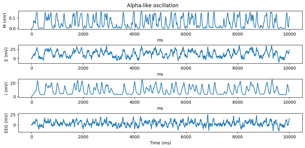
1) Alpha-like baseline oscillation

A single JR node with default parameters and moderate noisy drive exhibits an alpha-like rhythm (8–12 Hz).

• Model: brainmass.JansenRitModel(1) builds one node (one cortical column).

• Initialization: brainstate.nn.init_all_states(node) sets internal states consistently.

• Drive: mean 120 Hz with noise SD ≈ 30 Hz per sqrt(second), scaled per time step.

• Duration: 10 seconds.

# Alpha-like idle rhythm (baseline JR)
node = brainmass.JansenRitModel(1)
brainstate.nn.init_all_states(node)

def step_run(inp):
    eeg = node.update(E_inp=inp)
    return node.M.value, node.E.value, node.I.value, eeg

dt = brainstate.environ.get_dt()
indices = np.arange(int(10 * u.second / dt))
inputs = brainstate.random.normal(120., 30. / (dt / u.second) ** 0.5, indices.shape) * u.Hz
data = brainstate.transform.for_loop(step_run, inputs)
show(indices * dt, data, title='Alpha-like oscillation')

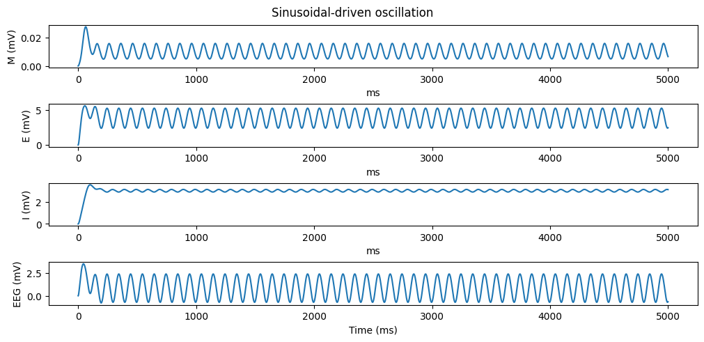
2) Sinusoidally driven/entrained oscillation

Adding a sinusoidal component to the input can entrain the JR node. Here we drive with a 10 Hz sinusoid around a baseline of ~80 Hz.

• Drive: inp(t) = 80 + 70 sin(2π f t) Hz with f = 10 Hz.

• Duration: 5 seconds.

node = brainmass.JansenRitModel(1)
brainstate.nn.init_all_states(node)
f_drive = 10. * u.Hz

def step_run(i):
    tt = i * dt
    inp = 80 + 70.0 * u.math.sin(2 * u.math.pi * f_drive * tt)
    eeg = node.update(E_inp=inp * u.Hz)
    return node.M.value, node.E.value, node.I.value, eeg

dt = brainstate.environ.get_dt()
indices = np.arange(int(5. * u.second / dt))
data = brainstate.transform.for_loop(step_run, indices)
show(indices * dt, data, title='Sinusoidal-driven oscillation')

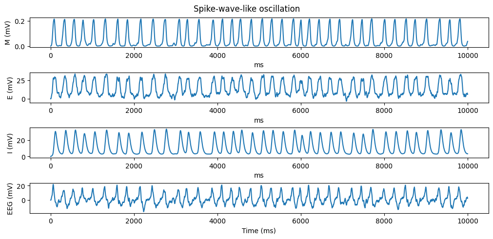
3) Spike–wave-like regime

Changing synaptic gains and time constants can push the node into a spike–wave-like regime reminiscent of epileptiform dynamics.

• Gains: increase excitatory gain Ae and reduce inhibitory gain Ai relative to typical JR defaults.

• Time constants: set inhibitory inverse time constant bi to 40 Hz (slower than the usual 50–100 Hz range), favoring prolonged inhibitory kinetics.

• Drive: mean 90 Hz with moderate noise.

• Duration: 10 seconds.

node = brainmass.JansenRitModel(1, Ae=4.5 * u.mV, Ai=18. * u.mV, bi=40. * u.Hz)
brainstate.nn.init_all_states(node)

def step_run(inp):
    eeg = node.update(E_inp=inp)
    return node.M.value, node.E.value, node.I.value, eeg

dt = brainstate.environ.get_dt()
indices = np.arange(int(10 * u.second / dt))
inputs = brainstate.random.normal(90., 10. / (dt / u.second) ** 0.5, indices.shape) * u.Hz
data = brainstate.transform.for_loop(step_run, inputs)
show(indices * dt, data, title='Spike-wave-like oscillation')

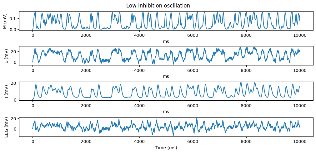
4) Reduced inhibition (disinhibited)

Lowering inhibitory strength typically increases oscillation amplitude and can shift frequency.

• Parameters: lower Ai and use bi = 40 Hz.

• Drive: mean 100 Hz with noise SD ≈ 20 Hz per sqrt(second).

• Duration: 10 seconds.

node = brainmass.JansenRitModel(1, Ai=15. * u.mV, bi=40. * u.Hz)
brainstate.nn.init_all_states(node)

def step_run(inp):
    eeg = node.update(E_inp=inp)
    return node.M.value, node.E.value, node.I.value, eeg

dt = brainstate.environ.get_dt()
indices = np.arange(int(10 * u.second / dt))
inputs = brainstate.random.normal(100., 20. / (dt / u.second) ** 0.5, indices.shape) * u.Hz
data = brainstate.transform.for_loop(step_run, inputs)
show(indices * dt, data, title='Low inhibition oscillation')

5) Irregular/noisy regime

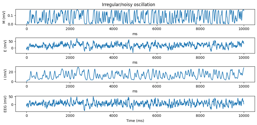
Increasing mean drive and noise level yields more irregular, broadband dynamics.

• Drive: mean 220 Hz with high noise SD ≈ 80 Hz per sqrt(second).

• Duration: 10 seconds.

node = brainmass.JansenRitModel(1)
brainstate.nn.init_all_states(node)

def step_run(inp):
    eeg = node.update(E_inp=inp)
    return node.M.value, node.E.value, node.I.value, eeg

dt = brainstate.environ.get_dt()
indices = np.arange(int(10 * u.second / dt))
inputs = brainstate.random.normal(220., 80. / (dt / u.second) ** 0.5, indices.shape) * u.Hz
data = brainstate.transform.for_loop(step_run, inputs)
show(indices * dt, data, title='Irregular/noisy oscillation')

Tips

• Change dt under the Setup cell to trade accuracy for speed (smaller dt is slower but more precise).

• Try different Ae, Ai, be, bi parameters when constructing JansenRitModel to explore bifurcations.

• Replace the noisy input with deterministic waveforms (ramps, chirps) to test entrainment and resonance.

• For reproducible noise, set the random seed if available in your brainstate version (e.g., brainstate.random.seed(0)).