Experiment Utilities with braintools

What is braintools?

braintools is the experiment-utility package in the BrainX ecosystem. It fills the practical gaps around neural dynamics models: task construction, input generation, parameter initialization, connectivity generation, file I/O, metric calculation, optimization, numerical integration, surrogate gradients, visualization, and spike encoding.

It is useful to think of braintools as the utility layer between a model and a full experiment. Packages such as brainstate and braincell focus on model states, neural dynamics, and simulation objects. braintools focuses on how those objects are organized into runnable, analyzable, and reproducible experiment workflows.

For deeper explanations, extended examples, and complete API references, see the full braintools documentation.

This tutorial follows a typical experiment workflow. It starts with setup, then introduces cognitive tasks, connectivity, file processing, initialization, input currents, metrics, optimization, numerical integration, surrogate gradients, visualization, and spike encoding. The final section combines several utilities into a compact end-to-end example.

Module overview

Module or utility	Main purpose	Example in this tutorial
braintools.cogtask	Build cognitive tasks, trial features, task phases, and sampled trial data	Use Feature and PerceptualDecisionMaking to generate inputs, targets, and trial metadata
braintools.conn	Generate neuron-to-neuron connectivity, sparse indices, weight matrices, and delays	Use AllToAll and FixedProb to build dense and random connectivity
braintools.file	Save and load parameters, checkpoints, and other pytree experiment artifacts	Use msgpack_save and msgpack_load to write and read a parameter dictionary
braintools.init	Initialize model parameters, state variables, synaptic weights, and readout weights	Use Normal, XavierNormal, and Constant to create arrays or connection weights
braintools.input	Generate common stimulus protocols and input currents, such as step, sinusoidal, noise, and Poisson spike inputs	Use step, sinusoidal, and poisson to create time-series inputs
braintools.metric	Compute neural activity metrics and machine-learning losses	Use firing_rate, cross entropy, and squared error to evaluate outputs
braintools.optim	Update trainable brainstate parameters	Use SGD to minimize a simple quadratic loss
braintools.quad	Provide numerical integration steps for ODEs, SDEs, DDEs, and IMEX systems	Use ode_rk4_step to integrate first-order decay dynamics
braintools.surrogate	Provide differentiable surrogate gradients for non-differentiable spike functions	Use a sigmoid spike function to inspect forward spikes and gradients
braintools.visualize	Plot raster plots, population activity, connectivity matrices, learning curves, and related figures	Use raster_plot and population_activity to visualize spike data
braintools.RateEncoder	Convert continuous values or input intensities into spike trains	Encode analog inputs as Bernoulli spike trains according to firing rate

Each section below corresponds to one utility category in the table. You can first scan the overview, then use the code examples to see where each tool fits in an experiment workflow.

1. Setup

The examples use short arrays and small time windows so the outputs are easy to inspect. Time-dependent utilities use brainunit units and the global brainstate time step. Random examples set explicit seeds when the API exposes one, so saved outputs are reproducible across documentation builds.

import tempfile
from pathlib import Path

import braintools
import brainstate
import brainunit as u
import jax
import jax.numpy as jnp
import matplotlib.pyplot as plt
import numpy as np

from braintools import cogtask, conn, file, init, input, metric, optim, quad, surrogate, visualize

brainstate.environ.set(dt=1.0 * u.ms)
brainstate.random.seed(0)

print(f"simulation dt: {brainstate.environ.get_dt()}")

simulation dt: 1. ms

2. Cognitive Tasks

Cognitive-task utilities describe experiments in terms of features, phases, and trial sampling. A feature specifies part of the input or target vector. A phase specifies an interval such as fixation, stimulus, delay, or response. A task combines these pieces into trial data that can drive a model.

Full documentation: Cognitive Tasks

# Feature sets map named task variables into slices of a trial input vector.
features = cogtask.Feature(1, "fixation") + cogtask.Feature(2, "motion") + cogtask.Feature(2, "choice")

print(features)
print(f"total input dimensions: {features.num}")
print(f"fixation slice: {features['fixation'].i}")
print(f"motion slice:   {features['motion'].i}")
print(f"choice slice:   {features['choice'].i}")

FeatureSet(names=['fixation', 'motion', 'choice'], nums=[1, 2, 2])
total input dimensions: 5
fixation slice: slice(0, 1, None)
motion slice:   slice(1, 3, None)
choice slice:   slice(3, 5, None)

# A ready-made perceptual decision-making task returns trial inputs, targets, and metadata.
task = cogtask.PerceptualDecisionMaking(
    t_fixation=20 * u.ms,
    t_stimulus=40 * u.ms,
    t_response=20 * u.ms,
    pop_per_choice=2,
    seed=0,
)

trial_inputs, trial_targets, trial_info = task.sample_trial(0)

print(task)
print(f"input shape:  {trial_inputs.shape}")
print(f"target shape: {trial_targets.shape}")
print(f"phases:       {trial_info['phase_history']}")
print(f"trial state:  {trial_info['trial_state']}")

Task(name=PerceptualDecisionMaking, inputs=5, outputs=3, output_mode=categorical)
input shape:  (80, 5)
target shape: (80,)
phases:       [('fixation', 0, 20), ('stimulus', 20, 60), ('response', 60, 80), ('Sequence', 60, 80)]
trial state:  {'trial_index': 0, 'ground_truth': Array(0, dtype=int32), 'coherence': Array(25.6, dtype=float32), 'stimulus_direction': Array(0., dtype=float32), 'output_mode': 'categorical'}

3. Synaptic Connectivity

Connectivity helpers create connection lists and optional weights or delays. The resulting ConnectionResult exposes sparse connection indices and conversion helpers such as weight2dense() and weight2csr(). In these arrays, pre_indices[k] -> post_indices[k] identifies one directed connection, while weights[k] stores the corresponding synaptic weight when a weight initializer is provided.

Full documentation: Synaptic Connectivity

all_to_all = conn.AllToAll(
    include_self_connections=False,
    weight=init.Constant(0.5),
)
result = all_to_all(pre_size=4, post_size=4)

print(f"shape: {result.shape}")
print(f"number of connections: {result.n_connections}")
print(f"pre indices:  {result.pre_indices}")
print(f"post indices: {result.post_indices}")
print("dense weights:")
print(result.weight2dense())

shape: (4, 4)
number of connections: 12
pre indices:  [0 0 0 1 1 1 2 2 2 3 3 3]
post indices: [1 2 3 0 2 3 0 1 3 0 1 2]
dense weights:
[[0.  0.5 0.5 0.5]
 [0.5 0.  0.5 0.5]
 [0.5 0.5 0.  0.5]
 [0.5 0.5 0.5 0. ]]

# Fixed-probability connectivity is useful for random network sketches.
# The seed is passed through the base Connectivity class for reproducible examples.
random_conn = conn.FixedProb(
    prob=0.35,
    allow_self_connections=False,
    weight=init.Constant(0.2),
    seed=1,
)
random_result = random_conn(pre_size=5, post_size=4)

print(f"random connection count: {random_result.n_connections}")
print("dense random weights:")
print(random_result.weight2dense())

random connection count: 8
dense random weights:
[[0.  0.  0.  0.2]
 [0.2 0.  0.2 0.2]
 [0.2 0.2 0.  0. ]
 [0.  0.  0.  0. ]
 [0.2 0.  0.2 0. ]]

4. File Processing

File utilities save and load pytrees such as parameter dictionaries. This is useful for checkpoints, initialized parameters, and experiment artifacts.

Full documentation: File Processing

params = {
    "weights": jnp.arange(6, dtype=jnp.float32).reshape(2, 3),
    "bias": jnp.array([0.1, -0.2], dtype=jnp.float32),
}

checkpoint_path = Path(tempfile.gettempdir()) / "braintools_tutorial_checkpoint.msgpack"
file.msgpack_save(str(checkpoint_path), params, overwrite=True, verbose=False)
loaded_params = file.msgpack_load(str(checkpoint_path), verbose=False)
checkpoint_path.unlink(missing_ok=True)

print("loaded keys:", sorted(loaded_params.keys()))
print("loaded weights:")
print(loaded_params["weights"])
print("loaded bias:", loaded_params["bias"])

loaded keys: ['bias', 'weights']
loaded weights:
[[0. 1. 2.]
 [3. 4. 5.]]
loaded bias: [ 0.1 -0.2]

5. Initialization

Initialization utilities create arrays for model parameters, synaptic weights, and readout layers. Distribution-based initializers are convenient for neuroscience-style parameters, while Xavier and Kaiming initializers are useful for trainable neural-network layers.

Full documentation: Initialization

rng = np.random.default_rng(0)

normal_weights = init.Normal(mean=0.0, std=0.1)((4, 3), rng=rng)
xavier_weights = init.XavierNormal()((4, 3), rng=rng)

print("Normal initializer")
print(f"  shape: {normal_weights.shape}")
print(f"  mean/std: {normal_weights.mean():.4f} / {normal_weights.std():.4f}")

print("Xavier normal initializer")
print(f"  shape: {xavier_weights.shape}")
print(f"  mean/std: {xavier_weights.mean():.4f} / {xavier_weights.std():.4f}")

Normal initializer
  shape: (4, 3)
  mean/std: 0.0022 / 0.0704
Xavier normal initializer
  shape: (4, 3)
  mean/std: -0.1338 / 0.5093

6. Input Current

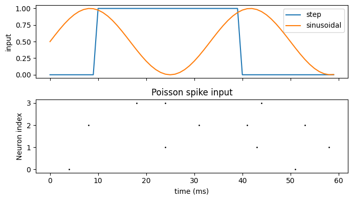
Input utilities generate common stimulation protocols: steps, ramps, oscillations, pulses, noise, and Poisson spike input. Unit-aware durations make the protocol align with the simulation time step. In practice, pass time arguments with units such as u.ms or u.Hz; this keeps protocol generation consistent with the global brainstate time step.

Full documentation: Input Current

step_current = input.step(
    amplitudes=[0.0, 1.0, 0.0],
    step_times=[0 * u.ms, 10 * u.ms, 40 * u.ms],
    duration=60 * u.ms,
)

sine_current = input.sinusoidal(
    amplitude=0.5,
    frequency=30 * u.Hz,
    duration=60 * u.ms,
    bias=True,
)

poisson_spikes = input.poisson(
    rate=40 * u.Hz,
    duration=60 * u.ms,
    n=4,
    seed=0,
)

time_ms = np.arange(step_current.shape[0])

fig, axes = plt.subplots(2, 1, figsize=(7, 4), sharex=True)
axes[0].plot(time_ms, step_current, label="step")
axes[0].plot(time_ms, sine_current, label="sinusoidal")
axes[0].set_ylabel("input")
axes[0].legend(loc="upper right")

visualize.raster_plot(time_ms, poisson_spikes, ax=axes[1], markersize=4, show=False)
axes[1].set_title("Poisson spike input")
axes[1].set_xlabel("time (ms)")
plt.tight_layout()
plt.show()

7. Metric Function

Metrics cover neural activity analysis and machine-learning objectives. The same module can compute firing rates, spike-train distances, classification losses, and regression errors.

Full documentation: Metric Function

spike_matrix = jnp.array(
    [
        [0, 1, 0, 0],
        [1, 0, 0, 1],
        [0, 0, 1, 0],
        [0, 0, 0, 0],
        [1, 0, 0, 0],
    ],
    dtype=jnp.float32,
)

population_rate = metric.firing_rate(spike_matrix, width=2.0, dt=1.0)
logits = jnp.array([[2.0, 0.0, -1.0], [0.1, 0.5, 1.2]])
labels = jnp.array([0, 2])
classification_loss = metric.softmax_cross_entropy_with_integer_labels(logits, labels)
regression_error = metric.squared_error(jnp.array([0.9, 1.8]), jnp.array([1.0, 2.0]), reduction="mean")

print("smoothed population firing rate:", population_rate)
print("classification loss per sample:", classification_loss)
print("mean squared error:", regression_error)

smoothed population firing rate: [0.375 0.5   0.375 0.25  0.125]
classification loss per sample: [0.16984604 0.6040188 ]
mean squared error: 0.025000012

8. Optimization

Optimization utilities provide familiar optimizers for trainable brainstate parameters. The example below minimizes a one-parameter quadratic loss with SGD.

Full documentation: Optimization

w = brainstate.ParamState(jnp.array(0.0), name="w")
optimizer = optim.SGD(lr=0.2)
optimizer.register_trainable_weights({"w": w})

history = []
for step in range(6):
    loss, grad = jax.value_and_grad(lambda value: (value - 3.0) ** 2)(w.value)
    optimizer.update({"w": grad})
    history.append((step, float(loss), float(w.value)))

for step, loss, value in history:
    print(f"step {step}: loss={loss:.4f}, w={value:.4f}")

step 0: loss=9.0000, w=1.2000
step 1: loss=3.2400, w=1.9200
step 2: loss=1.1664, w=2.3520
step 3: loss=0.4199, w=2.6112
step 4: loss=0.1512, w=2.7667
step 5: loss=0.0544, w=2.8600

9. Numerical Integration

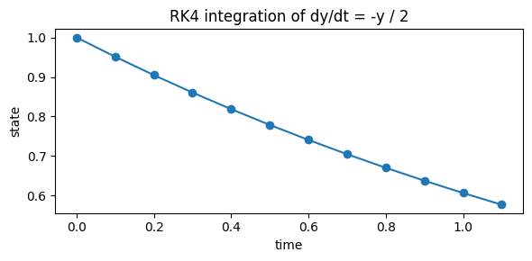
Numerical integration utilities implement single-step ODE, SDE, DDE, and IMEX methods. They are useful when you want a specific integration rule outside a larger simulator.

Full documentation: Numerical Integration

brainstate.environ.set(dt=0.1)

def decay(y, t):
    return -y / 2.0

y = jnp.array(1.0)
t = 0.0
trajectory = []
for _ in range(12):
    trajectory.append(float(y))
    y = quad.ode_rk4_step(decay, y, t)
    t += brainstate.environ.get_dt()

brainstate.environ.set(dt=1.0 * u.ms)

plt.figure(figsize=(6, 3))
plt.plot(np.arange(len(trajectory)) * 0.1, trajectory, marker="o")
plt.xlabel("time")
plt.ylabel("state")
plt.title("RK4 integration of dy/dt = -y / 2")
plt.tight_layout()
plt.show()

10. Surrogate Gradients

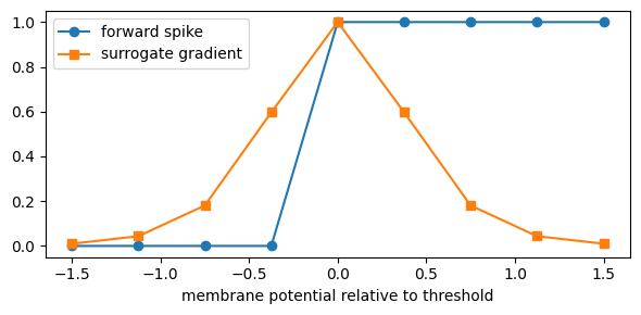
Binary spike functions are not differentiable in the usual sense. Surrogate-gradient functions keep the forward pass spike-like while supplying a smooth gradient to JAX autodiff.

Full documentation: Surrogate Gradients

x = jnp.linspace(-1.5, 1.5, 9)
spikes = surrogate.sigmoid(x, alpha=4.0)
grads = jax.grad(lambda z: jnp.sum(surrogate.sigmoid(z, alpha=4.0)))(x)

print("x:                 ", x)
print("forward spikes:    ", spikes)
print("surrogate gradient:", grads)

plt.figure(figsize=(6, 3))
plt.plot(x, spikes, "o-", label="forward spike")
plt.plot(x, grads, "s-", label="surrogate gradient")
plt.xlabel("membrane potential relative to threshold")
plt.legend()
plt.tight_layout()
plt.show()

x:                  [-1.5   -1.125 -0.75  -0.375  0.     0.375  0.75   1.125  1.5  ]
forward spikes:     [0. 0. 0. 0. 1. 1. 1. 1. 1.]
surrogate gradient: [0.00986604 0.04346492 0.18070664 0.59658587 1.         0.59658587
 0.18070662 0.04346485 0.00986586]

11. Visualization

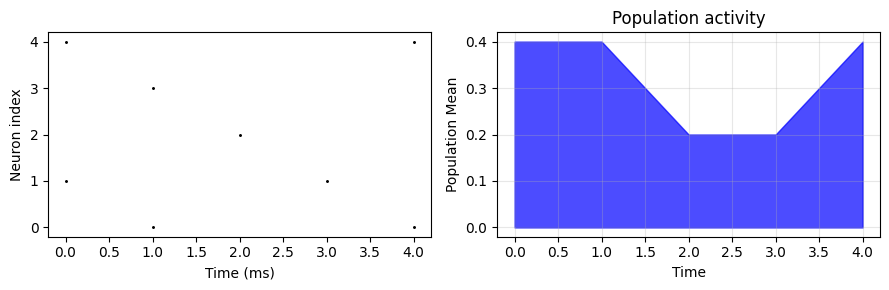
Visualization utilities provide ready-made plots for spike rasters, population activity, connectivity matrices, learning curves, trajectories, and related neural data views.

Full documentation: Visualization

example_spikes = np.array(
    [
        [0, 1, 0, 0, 1],
        [1, 0, 0, 1, 0],
        [0, 0, 1, 0, 0],
        [0, 1, 0, 0, 0],
        [1, 0, 0, 0, 1],
    ],
    dtype=float,
)
example_time = np.arange(example_spikes.shape[0])

fig, axes = plt.subplots(1, 2, figsize=(9, 3))
visualize.raster_plot(example_time, example_spikes, ax=axes[0], markersize=5, show=False)
visualize.population_activity(example_spikes, time=example_time, method="mean", ax=axes[1], title="Population activity")
plt.tight_layout()
plt.show()

12. Spike Encoding Methods

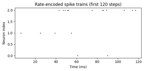
Spike encoders convert continuous values into spike trains. RateEncoder maps each input value to a firing rate in Hz, then samples Bernoulli spikes at each simulation step. With the default dt = 1 ms, a 100 Hz rate corresponds to a spike probability of about 0.1 per step.

The example below uses enough time steps to make the sampled spike probability close to the expected probability, while the raster plot only shows the first part of the generated train.

Full documentation: Spike Encoding Methods

brainstate.random.seed(1)

analog_values = jnp.array([0.1, 0.5, 0.9])
n_time = 1000
rate_gain_hz = 100.0

rate_encoder = braintools.RateEncoder(gain=rate_gain_hz, method="linear")
encoded_spikes = rate_encoder(analog_values, n_time=n_time)

# RateEncoder uses rate_hz * dt_ms / 1000 as the Bernoulli probability.
dt_ms = float(u.get_mantissa(brainstate.environ.get_dt()))
expected_probability = analog_values * rate_gain_hz * dt_ms / 1000.0
observed_probability = jnp.mean(encoded_spikes, axis=0)

print(f"analog values: {analog_values}")
print(f"encoded spike shape: {encoded_spikes.shape}")
print(f"expected spike probability per step: {expected_probability}")
print(f"observed spike probability over {n_time} steps: {observed_probability}")

plot_steps = 120
plt.figure(figsize=(6, 3))
visualize.raster_plot(
    np.arange(plot_steps),
    np.asarray(encoded_spikes[:plot_steps]),
    markersize=5,
    show=False,
)
plt.title(f"Rate-encoded spike trains (first {plot_steps} steps)")
plt.tight_layout()
plt.show()

analog values: [0.1 0.5 0.9]
encoded spike shape: (1000, 3)
expected spike probability per step: [0.01 0.05 0.09]
observed spike probability over 1000 steps: [0.013      0.042      0.09500001]

13. Mini Workflow

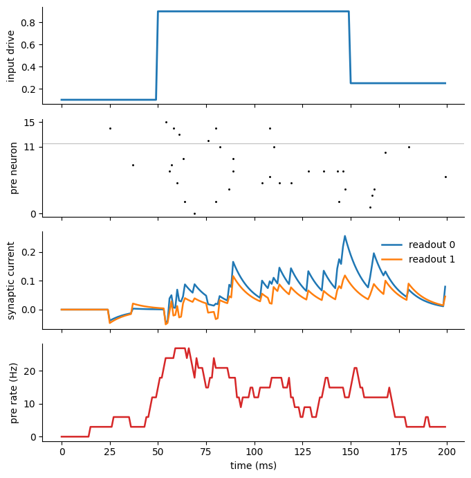
A typical experiment uses several braintools modules together. This mini workflow builds a time-varying input protocol, expands it into a small presynaptic population, encodes the drive values as spike trains, sends the spikes through an all-to-all projection, and summarizes the resulting readout currents.

The goal is to show how the utilities fit together in one compact pipeline: input generation, spike encoding, connectivity construction, simple synaptic filtering, metric calculation, and visualization. The same pattern can be extended to larger networks or replaced with more detailed neuron and synapse models when needed.

brainstate.random.seed(3)

dt = 1.0 * u.ms
brainstate.environ.set(dt=dt)
dt_ms = float(u.get_mantissa(dt))
n_steps = 200

# 1. Build a scalar input protocol with baseline, stimulus, and recovery phases.
stimulus = input.step(
    amplitudes=[0.1, 0.9, 0.25],
    step_times=[0 * u.ms, 50 * u.ms, 150 * u.ms],
    duration=n_steps * u.ms,
)
time_ms = np.arange(n_steps) * dt_ms
stimulus_array = jnp.asarray(stimulus[:n_steps])

# 2. Expand the scalar protocol into a small presynaptic population.
# The first 12 units follow excitatory-style weights; the last 4 use inhibitory-style weights.
n_stim_exc = 8
n_context_exc = 4
n_inh = 4
n_pre = n_stim_exc + n_context_exc + n_inh

stim_tuning = jnp.linspace(0.45, 1.0, n_stim_exc)
context_tuning = jnp.linspace(0.45, 0.8, n_context_exc)
inh_tuning = jnp.linspace(0.5, 0.9, n_inh)

stim_exc_drive = stimulus_array[:, None] * stim_tuning[None, :]
context_exc_drive = (0.35 + 0.10 * (1.0 - stimulus_array))[:, None] * context_tuning[None, :]
inh_drive = (0.20 + 0.25 * stimulus_array)[:, None] * inh_tuning[None, :]
presynaptic_drive = jnp.clip(
    jnp.concatenate([stim_exc_drive, context_exc_drive, inh_drive], axis=1),
    0.0,
    1.0,
)

# 3. Encode drives into presynaptic spikes with a rate-based encoder.
encoder = braintools.RateEncoder(gain=35.0, min_rate=2.0, method="linear")
presynaptic_spikes = encoder(presynaptic_drive, n_time=1)[0]

# 4. Convert spikes into a simple exponential synaptic trace before readout.
tau_syn_ms = 10.0
alpha = float(np.exp(-dt_ms / tau_syn_ms))
syn_state = jnp.zeros(n_pre, dtype=jnp.float32)
synaptic_trace = []
for spikes_t in presynaptic_spikes:
    syn_state = alpha * syn_state + spikes_t
    synaptic_trace.append(syn_state)
synaptic_trace = jnp.stack(synaptic_trace)

# 5. Create an all-to-all projection structure and apply two readout weight profiles.
connection_mask = jnp.asarray(
    conn.AllToAll(weight=init.Constant(1.0))(pre_size=n_pre, post_size=2).weight2dense()
)

stim_w0 = jnp.linspace(0.035, 0.075, n_stim_exc)
stim_w1 = jnp.linspace(0.015, 0.035, n_stim_exc)
context_w0 = jnp.linspace(0.015, 0.030, n_context_exc)
context_w1 = jnp.linspace(0.035, 0.060, n_context_exc)
inh_w0 = -jnp.linspace(0.025, 0.045, n_inh)
inh_w1 = -jnp.linspace(0.030, 0.055, n_inh)

readout_pattern = jnp.concatenate(
    [
        jnp.stack([stim_w0, stim_w1], axis=1),
        jnp.stack([context_w0, context_w1], axis=1),
        jnp.stack([inh_w0, inh_w1], axis=1),
    ],
    axis=0,
)
weights = connection_mask * readout_pattern
readout_current = synaptic_trace @ weights

# 6. Evaluate spike rates and readout currents.
presynaptic_rate = metric.firing_rate(presynaptic_spikes, width=20 * u.ms, dt=dt)
spike_counts = np.asarray(jnp.sum(presynaptic_spikes, axis=0))
observed_rates_hz = spike_counts * 1000.0 / (n_steps * dt_ms)
presynaptic_rate_np = np.asarray(presynaptic_rate)
readout_current_np = np.asarray(readout_current)

print(f"presynaptic drive:       {presynaptic_drive.shape}")
print(f"presynaptic spikes:      {presynaptic_spikes.shape}")
print(f"synaptic trace:          {synaptic_trace.shape}")
print(f"weights:                 {weights.shape}")
print(f"readout current:         {readout_current.shape}")
print(
    "observed pre rates:     "
    f"min={observed_rates_hz.min():.1f} Hz, "
    f"mean={observed_rates_hz.mean():.1f} Hz, "
    f"max={observed_rates_hz.max():.1f} Hz"
)
print(
    "population rate:        "
    f"min={presynaptic_rate_np.min():.1f} Hz, "
    f"mean={presynaptic_rate_np.mean():.1f} Hz, "
    f"max={presynaptic_rate_np.max():.1f} Hz"
)
print(
    "readout current ranges: "
    f"unit 0 [{readout_current_np[:, 0].min():.3f}, {readout_current_np[:, 0].max():.3f}], "
    f"unit 1 [{readout_current_np[:, 1].min():.3f}, {readout_current_np[:, 1].max():.3f}]"
)
print(f"excitatory-style weights nonnegative: {bool(jnp.all(weights[: n_stim_exc + n_context_exc] >= 0.0))}")
print(f"inhibitory-style weights nonpositive: {bool(jnp.all(weights[n_stim_exc + n_context_exc :] <= 0.0))}")

presynaptic drive:       (200, 16)
presynaptic spikes:      (200, 16)
synaptic trace:          (200, 16)
weights:                 (16, 2)
readout current:         (200, 2)
observed pre rates:     min=5.0 Hz, mean=11.2 Hz, max=30.0 Hz
population rate:        min=0.0 Hz, mean=11.7 Hz, max=28.1 Hz
readout current ranges: unit 0 [-0.044, 0.255], unit 1 [-0.051, 0.118]
excitatory-style weights nonnegative: True
inhibitory-style weights nonpositive: True

fig, axes = plt.subplots(4, 1, figsize=(7, 7), sharex=True)
axes[0].plot(time_ms, np.asarray(stimulus_array), color="tab:blue", linewidth=2)
axes[0].set_ylabel("input drive")

visualize.raster_plot(
    time_ms,
    np.asarray(presynaptic_spikes),
    ax=axes[1],
    markersize=5,
    xlabel=None,
    ylabel=None,
    show=False,
)
axes[1].axhline(n_stim_exc + n_context_exc - 0.5, color="0.75", linewidth=0.8)
axes[1].set_ylabel("pre neuron")
axes[1].set_yticks([0, n_stim_exc + n_context_exc - 1, n_pre - 1])
axes[1].set_ylim(-0.5, n_pre - 0.5)

axes[2].plot(time_ms, readout_current_np[:, 0], label="readout 0", linewidth=1.8)
axes[2].plot(time_ms, readout_current_np[:, 1], label="readout 1", linewidth=1.8)
axes[2].set_ylabel("synaptic current")
axes[2].legend(frameon=False, loc="upper right")

axes[3].plot(time_ms, presynaptic_rate_np, color="tab:red", linewidth=1.8)
axes[3].set_ylabel("pre rate (Hz)")
axes[3].set_xlabel("time (ms)")

for ax in axes:
    ax.spines["top"].set_visible(False)
    ax.spines["right"].set_visible(False)

plt.tight_layout()
plt.show()

14. Summary

This notebook introduced braintools as a practical utility layer for BrainX experiments. The examples showed how to generate cognitive-task trials, build synaptic connectivity, save and load pytrees, initialize parameters, create input currents, compute metrics, run optimization steps, apply numerical integration, use surrogate gradients, visualize neural activity, and encode continuous values as spike trains.

The main idea is that braintools helps connect the pieces around a simulation: experiment design, data generation, model support utilities, analysis, and visualization. This page is an entry point for the package. For deeper explanations, extended examples, and complete API references, follow the section-level links above or open the full braintools documentation.