Constructing LIF neuron model with brainstate

Welcome! This beginner-friendly tutorial will guide you through:

• Understanding the Leaky Integrate-and-Fire (LIF) neuron.

• Implementing LIF with brainstate.nn.Dynamics.

• Simulating with brainstate.transform.for_loop.

• Running small experiments (step response, tonic spiking, F–I curve).

Prerequisites:

• Basic Python. Some calculus intuition helps but is optional.

• brainstate and brainunit installed; this notebook uses unit-aware quantities (ms, mV, mA).

# Imports and environment setup
import braintools
import brainstate
import brainunit as u
import jax
import numpy as np
import matplotlib.pyplot as plt

# Global simulation step (time resolution)
brainstate.environ.set(dt=0.1 * u.ms)

LIF Basics

The LIF neuron approximates a neuron’s membrane as a leaky RC circuit. Its membrane potential V(t) obeys:

• ODE: dV/dt = (-(V - V_rest) + R I_in)/tau

• Parameters:

  • V_rest: resting potential (e.g., 0 mV here for simplicity).

  • R: membrane resistance (maps input current to a steady-state voltage).

  • tau: membrane time constant (how fast V relaxes).

  • I_in: input current.

Spiking and reset:

• When V crosses a threshold V_th, the neuron emits a spike.

• After spiking, V is reset (commonly to V_reset).

Discrete-time integration:

• We integrate with an exponential Euler step (brainstate.nn.exp_euler_step), equivalent to the exact solution for this linear ODE over one small time step dt.

• For constant input, the steady state is V_inf = V_rest + R I_in, and V(t + dt) = V_inf + (V(t) - V_inf) * exp(-dt/tau).

Implementing LIF with brainstate.nn.Dynamics

We implement a single-compartment LIF neuron.

from typing import Callable

class LIFDynamics(brainstate.nn.Dynamics):
    """
    A leaky integrate-and-fire neuron implemented as a Dynamics module.

    Parameters: R, tau, V_th, V_reset, V_rest, and a spike function.
    Soft reset subtracts (V_th - V_reset) when a spike occurs;
    Hard reset uses (V - V_reset), which resets exactly to V_reset.
    """
    def __init__(
        self,
        in_size: brainstate.typing.Size,
        R: brainstate.typing.ArrayLike = 1.0 * u.ohm,
        tau: brainstate.typing.ArrayLike = 5.0 * u.ms,
        V_th: brainstate.typing.ArrayLike = 1.0 * u.mV,
        V_reset: brainstate.typing.ArrayLike = 0.0 * u.mV,
        V_rest: brainstate.typing.ArrayLike = 0.0 * u.mV,
        V_initializer: Callable = braintools.init.Constant(0.0 * u.mV),
        spk_fun: Callable = braintools.surrogate.ReluGrad(),
        spk_reset: str = "soft",
        name: str | None = None,
    ):
        super().__init__(in_size, name=name)
        # Parameters (unit-aware)
        self.R = braintools.init.param(R, self.varshape)
        self.tau = braintools.init.param(tau, self.varshape)
        self.V_th = braintools.init.param(V_th, self.varshape)
        self.V_reset = braintools.init.param(V_reset, self.varshape)
        self.V_rest = braintools.init.param(V_rest, self.varshape)
        self.V_initializer = V_initializer
        # Spiking
        self.spk_fun = spk_fun
        self.spk_reset = spk_reset

    def init_state(self, batch_size: int | None = None, **kwargs):
        self.V = brainstate.HiddenState(
            braintools.init.param(self.V_initializer, self.varshape, batch_size)
        )

    def reset_state(self, batch_size: int | None = None, **kwargs):
        self.V.value = braintools.init.param(self.V_initializer, self.varshape, batch_size)

    def get_spike(self, V=None):
        V = self.V.value if V is None else V
        v_scaled = (V - self.V_th) / (self.V_th - self.V_reset)
        return self.spk_fun(v_scaled)

    def update(self, x=0.0 * u.mA):
        last_v = self.V.value
        spk = self.get_spike(last_v)
        # Reset policy
        V_th_or_v = self.V_th if self.spk_reset == 'soft' else jax.lax.stop_gradient(last_v)
        V = last_v - (V_th_or_v - self.V_reset) * spk
        # Dynamics integration by exponential Euler
        dv = lambda v: (-(v - self.V_rest) + self.R * x) / self.tau
        V = brainstate.nn.exp_euler_step(dv, V)
        self.V.value = V
        return self.get_spike(V)

# Create and initialize a neuron
lif = LIFDynamics(1)
brainstate.nn.init_all_states(lif)
lif

LIFDynamics(
  in_size=(1,),
  out_size=(1,),
  R=1. * ohm,
  tau=5. * msecond,
  V_th=1. * mvolt,
  V_reset=0. * mvolt,
  V_rest=0. * mvolt,
  V_initializer=Constant(value=0.0 * mvolt),
  spk_fun=ReluGrad(alpha=0.3, width=1.0),
  spk_reset=soft,
  V=HiddenState(
    value=~float32[1] * mvolt
  )
)

Code Walkthrough

• Parameters are registered with braintools.init.param to track shapes and units.

• Hidden state V holds the membrane potential and updates each step.

• get_spike(V): rescales (V - V_th) by (V_th - V_reset) and applies a surrogate spike function (here ReluGrad), enabling differentiable spikes for learning.

• Reset: soft subtracts (V_th - V_reset) * spk; hard subtracts (V - V_reset) * spk (i.e., set to V_reset when spiking).

• Integration: exp_euler_step advances V one dt under the environment’s time step.

Simulating with brainstate.transform.for_loop

We’ll write a small helper to run the neuron over a sequence of input currents, use indexing pattern with brainstate.environ.context(i=i).

def run_lif(lif_module, inputs):
    """Run the LIF over a 1D array of input currents.
    Returns membrane potentials and spikes over time.
    """
    lif_module.reset_state()
    idx = np.arange(len(inputs))

    def step(i, x):
        with brainstate.environ.context(i=i):
            s = lif_module(x)
            return lif_module.V.value, s

    V_seq, S_seq = brainstate.transform.for_loop(step, idx, inputs)
    return V_seq, S_seq

dt = brainstate.environ.get_dt()
dt

0.1 * msecond

Experiment 1: Subthreshold Step Response

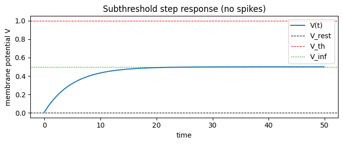
Use a constant current that keeps V_inf = V_rest + R I below V_th. We should see a smooth approach to V_inf without spiking.

n_time = 500
I_sub = 0.5 * u.mA  # V_inf = 0.5 mV < V_th = 1.0 mV
inputs = np.ones(n_time) * I_sub
V_sub, S_sub = run_lif(lif, inputs)
t = np.arange(n_time) * dt

plt.figure(figsize=(7, 3))
plt.plot(t, V_sub, label='V(t)')
plt.axhline(0.0 * u.mV, ls='--', c='k', lw=0.8, label='V_rest')
plt.axhline(1.0 * u.mV, ls='--', c='r', lw=0.8, label='V_th')
plt.axhline(0.5 * u.mV, ls=':', c='g', lw=1.0, label='V_inf')
plt.title('Subthreshold step response (no spikes)')
plt.xlabel('time')
plt.ylabel('membrane potential V')
plt.legend(loc='best')
plt.tight_layout()
plt.show()

Experiment 2: Suprathreshold Constant Current (Tonic Spiking)

Now choose a current with V_inf > V_th. The neuron should emit regular spikes. We’ll also estimate the firing rate from the simulated spikes.

n_time = 1500
I_sup = 1.5 * u.mA  # V_inf = 1.5 mV > V_th
inputs = np.ones(n_time) * I_sup
V_sup, S_sup = run_lif(lif, inputs)
t = np.arange(n_time) * dt

# Basic spike detection from surrogate output (>= 0.5 as spike)
spk_mask = np.asarray(S_sup) >= 0.5
spk_time, spk_indices = np.where(spk_mask)
spike_times = t[spk_time]

plt.figure(figsize=(8, 3))
plt.plot(t, V_sup, label='V(t)')
plt.plot(spike_times, V_sup[spk_time], 'rx', label='spikes')
plt.axhline(1.0 * u.mV, ls='--', c='r', lw=0.8, label='V_th')
plt.title('Suprathreshold input: tonic spiking')
plt.xlabel('time')
plt.ylabel('membrane potential V')
plt.legend(loc='best')
plt.tight_layout()
plt.show()

# Estimate firing rate from inter-spike intervals (ISI)
if spike_times.size > 1:
    isi = u.math.diff(spike_times)
    mean_isi = u.math.mean(isi)
    firing_rate = (1.0 / mean_isi).to(u.Hz)
    print('Mean ISI:', mean_isi)
    print('Estimated firing rate:', firing_rate)
else:
    print('No spikes detected — increase I_sup or duration.')

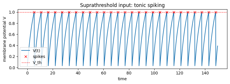
Mean ISI: 5.5 * msecond
Estimated firing rate: 181.81819 * hertz

Experiment 3: Soft vs Hard Reset

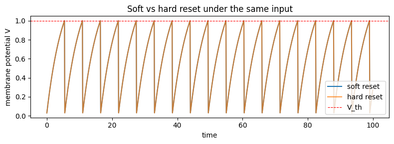
soft decreases V by (V_th - V_reset); hard resets directly to V_reset. Below we run both with the same current to compare trajectories.

lif_soft = LIFDynamics(1, spk_reset='soft')
lif_hard = LIFDynamics(1, spk_reset='hard')
brainstate.nn.init_all_states(lif_soft)
brainstate.nn.init_all_states(lif_hard)

n_time = 1000
inputs = np.ones(n_time) * (1.5 * u.mA)
V_soft, _ = run_lif(lif_soft, inputs)
V_hard, _ = run_lif(lif_hard, inputs)
t = np.arange(n_time) * dt

plt.figure(figsize=(8, 3))
plt.plot(t, V_soft, label='soft reset')
plt.plot(t, V_hard, label='hard reset', alpha=0.75)
plt.axhline(1.0 * u.mV, ls='--', c='r', lw=0.8, label='V_th')
plt.title('Soft vs hard reset under the same input')
plt.xlabel('time')
plt.ylabel('membrane potential V')
plt.legend(loc='best')
plt.tight_layout()
plt.show()

Experiment 4: F–I Curve (Firing Rate vs Current)

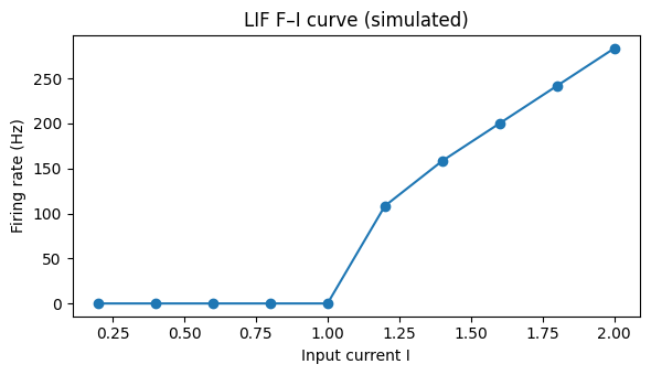
We sweep constant inputs and estimate the stationary firing rate at each level. This is a classic characterization for LIF neurons.

lif_fi = LIFDynamics(1)
brainstate.nn.init_all_states(lif_fi)

def estimate_rate(I_const, n_burn=300, n_eval=1200):
    # Simulate, drop initial transients (burn), then count spikes
    n_time = n_burn + n_eval
    inputs = np.ones(n_time) * I_const
    V, S = run_lif(lif_fi, inputs)
    spk = np.asarray(S[n_burn:]) >= 0.5
    n_spikes = spk.sum()
    T = n_eval * brainstate.environ.get_dt()
    rate = (n_spikes / (T / u.second)) * u.Hz
    return rate

curr_levels = np.linspace(0.2, 2.0, 10) * u.mA
rates = u.math.asarray([estimate_rate(I) for I in curr_levels])

plt.figure(figsize=(6, 3.5))
plt.plot(curr_levels, rates, 'o-')
plt.xlabel('Input current I')
plt.ylabel('Firing rate (Hz)')
plt.title('LIF F–I curve (simulated)')
plt.tight_layout()
plt.show()

Tips and Common Pitfalls

• Units matter: keep R, tau, V_*, and I consistent. brainunit helps track them.

• Time step dt: too large can distort dynamics or miss spikes; start with 0.1 ms.

• Always re-initialize or reset states before a new run (init_all_states once, reset_state per run).

• Surrogate spikes are differentiable; when just simulating, treat values >= 0.5 as spikes.

• Soft vs hard reset changes spike waveform and ISI slightly; both are common in literature.

Where To Go Next

• Add synaptic inputs and build small networks (brainstate.nn projections).

• Explore noise currents and refractory periods.

• Compare with conductance-based models (e.g., Hodgkin–Huxley) in the docs.