NEST-compatible point-neuron modeling with brainpy.state

The previous point-neuron tutorial introduced the BrainPy-style route: building networks directly from BrainX objects such as neurons, synapses, projections, inputs, and readouts. This tutorial introduces the other route provided by brainpy.state: NEST-compatible models.

NEST-compatible modeling is designed for users who know the NEST simulator, want to port NEST-style scripts, compare with NEST-style models, or prefer an explicit node/device/recorder workflow. It keeps familiar ideas such as creating model nodes, connecting populations, simulating a time window, and recording voltages or spikes. At the same time, the model stays inside the BrainX ecosystem: values use explicit physical units from brainunit, simulation state is managed by brainpy.state and brainstate, and computations use JAX-compatible arrays.

For the complete model catalog, API reference, validation notes, and guides for both BrainPy-style and NEST-compatible modeling, read the full brainpy.state documentation.

You will learn how to:

1. create NEST-compatible model nodes and recording devices with Simulator.create();

2. connect populations, projections, and recorders with Simulator.connect();

3. simulate a network for a unit-aware duration with Simulator.simulate();

4. read membrane traces and spike events from the returned result object;

5. extend the same workflow from one neuron to connection rules and a small excitatory/inhibitory network.

Setup

Enable JAX x64 before importing brainpy.state, then give each Simulator an explicit unit-aware time step. The examples below use milliseconds, picoamperes, and millivolts from brainunit.

import jax

import numpy as np
import matplotlib.pyplot as plt

import brainunit as u
import brainpy.state as bp

1. Create: model nodes

Simulator.create() is the brainpy.state counterpart of NEST’s Create. It returns a NodeView, which is a handle to the created population or device.

The example below creates one iaf_psc_alpha neuron. Parameters use NEST-compatible names such as I_e, V_th, V_reset, and E_L, while values remain explicit brainunit quantities.

sim = bp.Simulator(dt=0.1 * u.ms)

neuron = sim.create(
    bp.iaf_psc_alpha,
    params={
        "I_e": 376.0 * u.pA,
        "V_th": -55.0 * u.mV,
        "V_reset": -70.0 * u.mV,
        "E_L": -70.0 * u.mV,
    },
)

print(neuron)
print(f"number of nodes = {len(neuron)}")

<brainpy.state.NodeView object at 0x000001507C3DA110>
number of nodes = 1

2. Connect: recording devices

Recording devices follow NEST’s connection direction:

• a voltmeter observes a neuron, so connect voltmeter -> neuron;

• a spike_recorder receives spike events, so connect neuron -> spike_recorder.

The same Simulator.connect() method registers either a projection or a recorder tap depending on the source and target types.

vm = sim.create(bp.voltmeter, interval=0.1 * u.ms)
sr = sim.create(bp.spike_recorder)

sim.connect(vm, neuron)      # voltmeter observes the neuron
sim.connect(neuron, sr)      # spike_recorder receives emitted spikes

print("recorders are connected")

recorders are connected

3. Simulate: run the model

Simulator.simulate() is the explicit runner. It returns a SimulationResult object with helper methods for recorded variables:

• trace(recorder, "V_m") returns a membrane-potential trace from a voltmeter or multimeter;

• spikes(recorder) returns a time-by-node spike matrix;

• n_events(recorder) counts recorded spikes;

• rate(recorder) reports the mean firing rate in spikes per second.

result = sim.simulate(80.0 * u.ms)

V_m = result.trace(vm, "V_m")
spikes = result.spikes(sr)
times = result.times

print(f"V_m shape     = {V_m.shape}")
print(f"spikes shape  = {spikes.shape}")
print(f"spike count   = {result.n_events(sr)}")
print(f"firing rate   = {result.rate(sr):.2f} Hz")

V_m shape     = (800, 1)
spikes shape  = (800, 1)
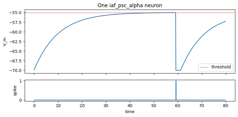
spike count   = 1
firing rate   = 12.50 Hz

4. Record: visualize traces and events

The result object separates simulation from analysis. Once the run has finished, use recorder handles to extract arrays and plot them with ordinary Python tools. This mirrors the NEST habit of attaching devices first and reading them after Simulate.

fig, axes = plt.subplots(2, 1, figsize=(8, 4), sharex=True, height_ratios=[3, 1])

axes[0].plot(times, V_m[:, 0])
axes[0].axhline(-55.0 * u.mV, color="tab:red", ls="--", lw=0.9, label="threshold")
axes[0].set_ylabel("V_m")
axes[0].set_title("One iaf_psc_alpha neuron")
axes[0].legend(loc="best")

axes[1].plot(times, spikes[:, 0], drawstyle="steps-post")
axes[1].set_ylabel("spike")
axes[1].set_xlabel("time")

plt.tight_layout()
plt.show()

5. NodeView algebra: populations, slices, and groups

A NodeView can refer to a full population, a slice of one population, or a concatenation of several views. This gives you a compact way to express NEST-like population algebra while keeping Python objects explicit.

A practical constraint: a single spike_recorder records one population segment. If you concatenate two populations, use one recorder per population when you want spike recordings from both groups.

pop_sim = bp.Simulator(dt=0.1 * u.ms)

exc = pop_sim.create(bp.iaf_psc_alpha, 6, params={"I_e": 400.0 * u.pA})
inh = pop_sim.create(bp.iaf_psc_alpha, 3, params={"I_e": 360.0 * u.pA})

first_two_exc = exc[:2]
all_neurons = exc + inh

print(f"exc size           = {len(exc)}")
print(f"inh size           = {len(inh)}")
print(f"first_two_exc size = {len(first_two_exc)}")
print(f"combined size      = {len(all_neurons)}")

exc size           = 6
inh size           = 3
first_two_exc size = 2
combined size      = 9

6. Connect: population projections

Connection rules are passed to sim.connect() through the rule argument. The common pattern is:

sim.connect(pre, post, rule=..., weight=..., delay=..., seed=...)

Positive weights drive excitatory current channels, while negative weights drive inhibitory current channels for current-based NEST-compatible neurons. Delays are unit-aware time quantities.

For known dense examples, the default communication path is fine. For larger sparse networks, comm="sparse" routes event delivery through sparse communication while preserving the same high-level connect() interface.

# E -> I: sparse random excitatory projection.
pop_sim.connect(
    exc,
    inh,
    rule=bp.pairwise_bernoulli(0.5),
    weight=20.0 * u.pA,
    delay=1.0 * u.ms,
    seed=1,
)

# I -> E: sparse random inhibitory projection.
pop_sim.connect(
    inh,
    exc,
    rule=bp.pairwise_bernoulli(0.5),
    weight=-45.0 * u.pA,
    delay=1.0 * u.ms,
    seed=2,
)

print("E/I projections are connected")

E/I projections are connected

Deterministic connection rules

The same interface also covers deterministic rules. This cell uses a separate simulator only to show the API shape without interfering with the E/I example above.

rule_sim = bp.Simulator(dt=0.1 * u.ms)
pre = rule_sim.create(bp.iaf_psc_alpha, 3, params={"I_e": 380.0 * u.pA})
post = rule_sim.create(bp.iaf_psc_alpha, 3)

one_to_one_proj = rule_sim.connect(
    pre,
    post,
    rule=bp.one_to_one,
    weight=15.0 * u.pA,
    delay=1.0 * u.ms,
)

all_to_all_proj = rule_sim.connect(
    pre,
    post,
    rule=bp.all_to_all,
    weight=5.0 * u.pA,
    delay=1.0 * u.ms,
)

print(type(one_to_one_proj).__name__)
print(type(all_to_all_proj).__name__)

EventProjection
EventProjection

7. Record: a small E/I network

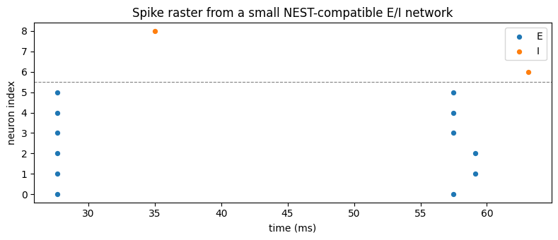
Now attach one spike recorder to the excitatory population and one to the inhibitory population. This keeps each recorder tied to a single population segment, which is the supported recording layout for spike recorders.

exc_rec = pop_sim.create(bp.spike_recorder)
inh_rec = pop_sim.create(bp.spike_recorder)

pop_sim.connect(exc, exc_rec)
pop_sim.connect(inh, inh_rec)

net_result = pop_sim.simulate(80.0 * u.ms)

exc_spikes = net_result.spikes(exc_rec)
inh_spikes = net_result.spikes(inh_rec)

print(f"exc_spikes shape = {exc_spikes.shape}")
print(f"inh_spikes shape = {inh_spikes.shape}")
print(f"exc events       = {net_result.n_events(exc_rec)}")
print(f"inh events       = {net_result.n_events(inh_rec)}")
print(f"exc rate         = {net_result.rate(exc_rec):.2f} Hz")
print(f"inh rate         = {net_result.rate(inh_rec):.2f} Hz")

exc_spikes shape = (800, 6)
inh_spikes shape = (800, 3)
exc events       = 12
inh events       = 2
exc rate         = 25.00 Hz
inh rate         = 8.33 Hz

def raster_points(spike_matrix, offset=0):
    t_idx, neuron_idx = np.where(np.asarray(spike_matrix) > 0)
    return t_idx, neuron_idx + offset

exc_t, exc_id = raster_points(exc_spikes, offset=0)
inh_t, inh_id = raster_points(inh_spikes, offset=len(exc))

time_values = np.asarray(net_result.times.to_decimal(u.ms))

plt.figure(figsize=(8, 3.5))
if len(exc_t):
    plt.scatter(time_values[exc_t], exc_id, s=18, label="E", color="tab:blue")
if len(inh_t):
    plt.scatter(time_values[inh_t], inh_id, s=18, label="I", color="tab:orange")

plt.axhline(len(exc) - 0.5, color="0.5", lw=0.8, ls="--")
plt.xlabel("time (ms)")
plt.ylabel("neuron index")
plt.title("Spike raster from a small NEST-compatible E/I network")
plt.legend(loc="upper right")
plt.tight_layout()
plt.show()

8. Translate NEST scripts carefully

Quick translation map

NEST concept	brainpy.state pattern	Notes
nest.Create("iaf_psc_alpha", n, params=...)	sim.create(bp.iaf_psc_alpha, n, params=...)	Model names are Python classes, not strings.
nest.Connect(pre, post, conn_spec, syn_spec)	sim.connect(pre, post, rule=..., weight=..., delay=...)	Connection rule and synaptic parameters are explicit keyword arguments.
nest.Simulate(t)	sim.simulate(t * u.ms)	Duration is a brainunit quantity.
voltmeter -> neuron	sim.connect(vm, neuron)	Analog recorders observe the target population.
neuron -> spike_recorder	sim.connect(neuron, sr)	Spike recorders receive events from one population segment.
NodeCollection slicing	node_view[:k], view_a + view_b	Concatenated views are useful for population algebra, but some devices require one segment.

Porting cautions

Area	What changes in BrainX	Practical guidance
Units	Physical quantities are explicit objects, not bare numbers.	Write 20.0 * u.pA, 1.0 * u.ms, and -55.0 * u.mV; convert deliberately when plotting or exporting.
Model identifiers	Models are imported Python classes/functions.	Use bp.iaf_psc_alpha, bp.voltmeter, and bp.spike_recorder instead of string model names.
Device direction	Recorder connections keep NEST-style direction.	Connect voltmeter -> neuron for analog traces and neuron -> spike_recorder for spikes.
Recorder scope	Spike recorders are tied to a population segment.	Use separate recorders for excitatory and inhibitory groups when you need separate raster data.
JAX execution	Arrays and simulations are JAX-compatible and may be compiled internally.	Keep model construction outside repeated simulation loops; pass changing inputs and parameters explicitly.
Validation	Compatibility focuses on documented semantics, not byte-for-byte equality with every NEST run.	Check units, time step, delays, seeds, and documented model assumptions when comparing results.

For model physiology, use the upstream NEST model documentation. For brainpy.state, focus on the Python API, unit handling, simulator semantics, and documented validation status.

9. Summary

The NEST-compatible layer in brainpy.state gives you a familiar workflow while staying inside the BrainX/JAX ecosystem:

1. create model nodes and devices with Simulator.create();

2. wire populations, projections, and recorders with Simulator.connect();

3. run a simulation window with Simulator.simulate();

4. inspect traces and events with SimulationResult.trace(), spikes(), n_events(), and rate().

When porting NEST scripts, preserve the workflow but adopt BrainX idioms: explicit units, Python model objects, JAX-compatible arrays, and stateful simulation objects managed by brainpy.state and brainstate.