

Spike Encoding#
Spiking networks need their inputs as spikes. braintools.spike provides ten encoders that turn numbers or time series into spike trains (or, in one case, a current). They fall into four groups:
Group |
Encoders |
Information is carried by |
|---|---|---|
Rate codes (stochastic) |
|
how often a neuron fires |
Timing codes (deterministic) |
|
when, in what order, or how many times a neuron fires |
Signal codes |
|
changes of a time series, or a constant current |
Symbol codes |
|
which neuron fires, with a fixed spike pattern per symbol |
Conventions shared by all encoders:
the time step comes from
brainstate.environ(set it with a unit, e.g.0.1 * u.ms);n_timeis the number of time steps; outputs have shape(n_time, *data.shape)(the population encoder adds a neuron axis);stochastic encoders draw from
brainstate.random, so seed it withbrainstate.random.seed(...);a firing rate is recovered from a spike matrix as
spikes.mean(axis=0) / dt.
1. Setup#
import brainstate
import brainunit as u
import jax.numpy as jnp
import matplotlib.pyplot as plt
import numpy as np

import braintools

dt = 0.1 * u.ms
brainstate.environ.set(dt=dt)
brainstate.random.seed(0)
dt_s = dt.to_decimal(u.second)


def raster(ax, spikes, title):
    s = np.asarray(spikes)
    t_idx, n_idx = np.nonzero(s)
    ax.plot(t_idx * dt.to_decimal(u.ms), n_idx, "|", ms=8, color="k")
    ax.set_title(title, fontsize=10)
    ax.set_xlabel("time (ms)")
    ax.set_ylim(-0.5, s.shape[1] - 0.5)
2. Rate Codes#
RateEncoder(gain, method, min_rate, max_rate) maps an input \(x \in [0, 1]\) to a rate between min_rate and max_rate (default gain), linearly, through \((e^x - 1)/(e - 1)\), or through \(\sqrt x\), then fires in each step with probability \(\text{rate} \cdot dt\). PoissonEncoder takes rates in Hz directly (or \(x \cdot\) max_rate with normalize=True) and returns 1 when a Poisson draw with mean \(\text{rate}\cdot dt\) is positive, so the firing probability per step is \(1 - e^{-\text{rate}\cdot dt}\). The two agree at low rates; the Poisson version saturates more smoothly at high ones.
n = 400_000  # 40 s, so the estimates are within about 1 Hz
x = jnp.array([0.2, 0.5, 0.8])
print("RateEncoder, gain 100 Hz:")
for method, f in [("linear", lambda v: v), ("exponential", lambda v: (np.exp(v) - 1) / (np.e - 1)), ("sqrt", np.sqrt)]:
    measured = braintools.spike.RateEncoder(gain=100.0, method=method)(x, n).mean(axis=0) / dt_s
    print(f"  {method:11s} measured {np.round(np.asarray(measured), 1)} Hz, expected {np.round(100 * f(np.asarray(x)), 1)} Hz")

rates = jnp.array([20.0, 200.0, 2000.0])
p_spike = braintools.spike.PoissonEncoder()(rates, n).mean(axis=0)
print("\nPoissonEncoder, P(spike per step):")
print("  measured ", np.round(np.asarray(p_spike), 4))
print("  1-exp(-r dt)", np.round(1 - np.exp(-np.asarray(rates) * dt_s), 4), " vs  r*dt", np.asarray(rates) * dt_s)
RateEncoder, gain 100 Hz:
  linear      measured [19.7 48.5 81. ] Hz, expected [20. 50. 80.] Hz
  exponential measured [12.8 37.  71.6] Hz, expected [12.9 37.8 71.3] Hz
  sqrt        measured [46.3 70.4 92. ] Hz, expected [44.7 70.7 89.4] Hz
PoissonEncoder, P(spike per step):
  measured  [0.0021 0.0198 0.1822]
  1-exp(-r dt) [0.002  0.0198 0.1813]  vs  r*dt [0.002      0.02       0.19999999]
BernoulliEncoder(scale) fires with probability \(x \cdot \text{scale}\) per time step, independently of dt: the same input gives ten times the rate in Hz if dt is ten times smaller. Use it when the probability per step is what you want to control (for example, image pixels presented for a fixed number of steps).
for step in [0.1 * u.ms, 1.0 * u.ms]:
    with brainstate.environ.context(dt=step):
        s = braintools.spike.BernoulliEncoder(scale=0.5)(jnp.array([0.4]), 50_000)
        print(f"dt = {step}: P(spike) {float(s.mean()):.3f} (0.4 * 0.5 = 0.2), rate {float(s.mean()) / step.to_decimal(u.second):.0f} Hz")
dt = 0.1 ms: P(spike) 0.199 (0.4 * 0.5 = 0.2), rate 1994 Hz
dt = 1. ms: P(spike) 0.201 (0.4 * 0.5 = 0.2), rate 201 Hz
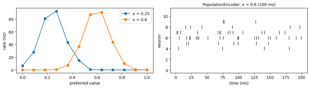
PopulationEncoder(n_neurons, min_val, max_val, sigma, max_rate) represents a scalar with a population of neurons whose preferred values are evenly spaced; neuron \(i\) fires at \(\text{max\_rate}\cdot e^{-(x - c_i)^2 / 2\sigma^2}\). The output has shape (n_time, n_neurons) for a scalar input. The value can be read back from the spike counts, for example with a population-vector average of the preferred values:
pop = braintools.spike.PopulationEncoder(n_neurons=12, min_val=0.0, max_val=1.0, sigma=0.1, max_rate=100.0)
centers = np.asarray(pop.centers)
fig, axes = plt.subplots(1, 2, figsize=(11, 3.2))
for value in [0.25, 0.6]:
    spikes = pop(value, 20_000)  # 2 s
    counts = np.asarray(spikes.sum(axis=0))
    decoded = (counts * centers).sum() / counts.sum()
    print(f"input {value:.2f}: decoded {decoded:.3f}, spikes per neuron {counts.astype(int)}")
    axes[0].plot(centers, counts / 2.0, "o-", label=f"x = {value}")
axes[0].set_xlabel("preferred value")
axes[0].set_ylabel("rate (Hz)")
axes[0].legend()
raster(axes[1], pop(0.6, 2000), "PopulationEncoder, x = 0.6 (200 ms)")
axes[1].set_ylabel("neuron")
fig.tight_layout()
plt.show()
input 0.25: decoded 0.245, spikes per neuron [ 13  56 161 185  86  30   1   0   0   0   0   0]
input 0.60: decoded 0.597, spikes per neuron [  0   0   0   1  15  74 174 181  87  20   1   0]
3. Timing Codes#
LatencyEncoder gives every feature exactly one spike, earlier for larger values. n_time is the window in steps (a quantity is converted with dt; the default window is tau).
method='linear': \(t = t_0 + T(1 - x)\).method='log': \(t = t_0 + T \log\frac{x}{x - \theta}\), the time a leaky integrator driven by \(x\) needs to reach threshold \(\theta\).normalize=Truechooses \(T\) so the slowest input (\(x = 0\) for linear, \(x = \theta\) for log) fires in the last step.normalize=Falseuses the physical time constanttauinstead and drops spikes that would fall after the window.clip=Truesilences inputs belowthreshold.
x = jnp.array([0.0, 0.25, 0.5, 0.75, 1.0])
lin = braintools.spike.LatencyEncoder(method="linear", normalize=True)(x, n_time=101)
print("linear, normalized, 101 steps:      spike step", np.asarray(jnp.argmax(lin, axis=0)))

log = braintools.spike.LatencyEncoder(method="log", normalize=True, threshold=0.05)(jnp.array([0.05, 0.1, 0.25, 0.5, 1.0]), n_time=101)
print("log, normalized, x = .05 .. 1:      spike step", np.asarray(jnp.argmax(log, axis=0)))

phys = braintools.spike.LatencyEncoder(method="linear", normalize=False, tau=5 * u.ms)(x, n_time=3 * u.ms)
print(f"linear, tau = 5 ms, 3 ms window ({phys.shape[0]} steps): spikes per feature {np.asarray(phys.sum(0)).astype(int)} "
      f"(x = 0 and 0.25 would fire at 5 and 3.75 ms)")
linear, normalized, 101 steps:      spike step [100  75  50  25   0]
log, normalized, x = .05 .. 1:      spike step [100   5   2   1   0]
linear, tau = 5 ms, 3 ms window (30 steps): spikes per feature [0 0 1 1 1] (x = 0 and 0.25 would fire at 5 and 3.75 ms)
The log code is strongly compressed: inputs well above threshold all fire within the first few steps, and resolution is concentrated just above the threshold. Use 'linear' when inputs are spread evenly over \([0, 1]\).
RankOrderEncoder also emits one spike per feature, larger values first. With use_values=True the time is proportional to \(1 - x\) after rescaling the vector to \([0, 1]\) (equal values fire together); with use_values=False only the rank matters and spikes are evenly spaced. invert=True reverses the order.
v = jnp.array([0.1, 0.11, 0.9, 0.91, 0.5])
by_value = jnp.argmax(braintools.spike.RankOrderEncoder(use_values=True)(v, n_time=50), axis=0)
by_rank = jnp.argmax(braintools.spike.RankOrderEncoder(use_values=False)(v, n_time=50), axis=0)
print("values:          ", np.asarray(v))
print("use_values=True: ", np.asarray(by_value), "(close values fire together)")
print("use_values=False:", np.asarray(by_rank), "(evenly spaced by rank)")
values:           [0.1  0.11 0.9  0.91 0.5 ]
use_values=True:  [49 48  0  0 24] (close values fire together)
use_values=False: [39 29  9  0 19] (evenly spaced by rank)
SpikeCountEncoder(max_spikes, distribution) fires exactly \(\lfloor x \cdot \text{max\_spikes}\rfloor\) times in the window, spread evenly ('uniform') or at random distinct steps ('random'). With normalize=True (default) inputs are clipped to \([0, 1]\); a window can hold at most n_time spikes.
x = jnp.array([0.0, 0.35, 0.7, 1.0])
for dist in ["uniform", "random"]:
    s = braintools.spike.SpikeCountEncoder(max_spikes=10, distribution=dist)(x, n_time=200)
    print(f"{dist:7s} counts {np.asarray(s.sum(axis=0)).astype(int)}  (floor(10 x) = {np.floor(10 * np.asarray(x)).astype(int)})")
uniform counts [ 0 3 7 10] (floor(10 x) = [ 0 3 7 10])
random counts [ 0 3 7 10] (floor(10 x) = [ 0 3 7 10])
4. Signal Codes#
DeltaEncoder(threshold) encodes a time series (n_time, *features) by send-on-delta modulation: it keeps a reference level, emits an event when the signal has moved threshold away from it, and resets the reference to the current value. Events are \(+1\) for increases and \(-1\) for decreases (ON/OFF), or 0/1 with absolute=True or positive_only=True. With normalize=True each feature is first rescaled to \([0, 1]\) over time, so threshold is a fraction of its range.
Because every event marks a change of about threshold, the signal can be approximately reconstructed by summing the events:
t = np.arange(4000) * dt.to_decimal(u.ms)  # 400 ms
signal = 0.5 + 0.3 * np.sin(2 * np.pi * t / 200) + 0.15 * np.sin(2 * np.pi * t / 37)
events = np.asarray(braintools.spike.DeltaEncoder(threshold=0.05, normalize=False)(jnp.asarray(signal)))
reconstruction = signal[0] + 0.05 * np.cumsum(events)
print(f"{int(np.abs(events).sum())} events ({int((events > 0).sum())} ON, {int((events < 0).sum())} OFF); "
      f"max |reconstruction error| {np.abs(reconstruction - signal).max():.3f} (threshold 0.05)")

fig, ax = plt.subplots(figsize=(10, 3))
ax.plot(t, signal, lw=1, label="signal")
ax.step(t, reconstruction, where="post", lw=1, label="signal[0] + 0.05 * cumsum(events)")
on, off = events > 0, events < 0
ax.plot(t[on], signal[on], "^", ms=4, color="C2", label="ON")
ax.plot(t[off], signal[off], "v", ms=4, color="C3", label="OFF")
ax.set_xlabel("time (ms)")
ax.legend(fontsize=8)
plt.show()
105 events (51 ON, 54 OFF); max |reconstruction error| 0.068 (threshold 0.05)
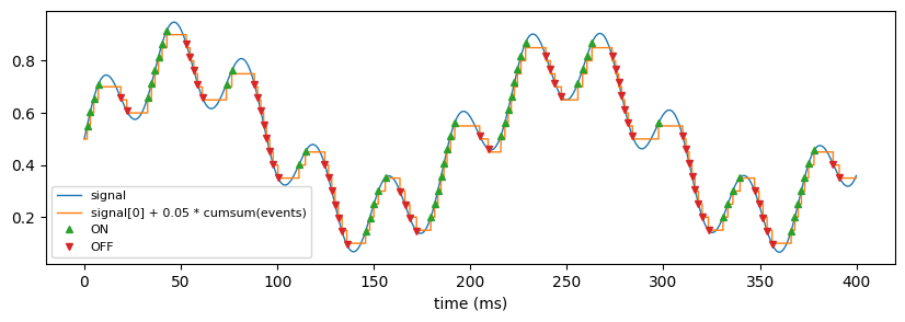
Between events the signal stays within one threshold of the reference. The summed reconstruction drifts slightly beyond that: at each event the reference jumps to the actual value, which has moved a little more than threshold, while the reconstruction adds exactly threshold. The overshoot is at most one step’s change of the signal, so it stays small when the signal is smooth relative to dt. Event cameras (DVS) have the same property. A finer threshold gives a more faithful code at the price of more events.
StepCurrentEncoder(current_scale, offset) does not produce spikes: it returns the constant current \(x \cdot \text{current\_scale} + \text{offset}\) in every step, for injection into a neuron model that then produces the spikes. The values are plain numbers; multiply by a unit when the model expects a quantity. Here the currents drive a leaky integrate-and-fire neuron, whose firing rate grows with the input:
x = jnp.array([0.1, 0.3, 0.6, 1.0])
I = braintools.spike.StepCurrentEncoder(current_scale=0.5, offset=0.0)(x, n_time=5000) * u.nA  # 500 ms
tau, R, E_L, V_th = 20 * u.ms, 100 * u.Mohm, -70 * u.mV, -50 * u.mV
V = u.math.full(4, -70.0) * u.mV
count = np.zeros(4, dtype=int)
for I_t in I:
    V = V + dt / tau * (-(V - E_L) + R * I_t)
    fired = np.asarray(V >= V_th)
    count += fired
    V = u.math.where(fired, E_L, V)
print("input:", np.asarray(x), " current (nA):", np.asarray(I[0].to_decimal(u.nA)), " rate (Hz):", count / 0.5)
input: [0.1 0.3 0.6 1. ] current (nA): [0.05 0.15 0.3 0.5 ] rate (Hz): [ 0. 0. 44. 98.]
Inputs whose current stays below rheobase (\((V_{th} - E_L)/R = 0.2\) nA) produce no spikes at all: a current code adds the neuron’s own nonlinearity on top of the encoding.
5. Symbol Codes#
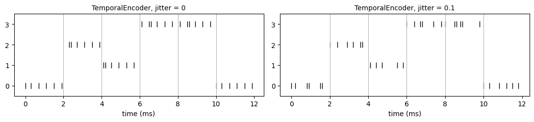
TemporalEncoder(n_patterns, pattern_length, jitter) encodes a sequence of integer symbols. Each symbol occupies pattern_length steps; during that slot, the neuron with the symbol’s index fires a fixed pattern of spikes (about 30 % of the slot), shifted by \(2 \times\) symbol index, with Gaussian jitter of jitter * pattern_length steps. The output has shape (len(sequence) * pattern_length, n_patterns); the identity of the active neuron is what carries the symbol.
sequence = jnp.array([0, 2, 1, 3, 3, 0])
clean = braintools.spike.TemporalEncoder(n_patterns=4, pattern_length=20, jitter=0.0)(sequence)
noisy = braintools.spike.TemporalEncoder(n_patterns=4, pattern_length=20, jitter=0.1)(sequence)
print("output shape:", clean.shape)
decoded = np.asarray(clean.reshape(len(sequence), 20, 4).sum(axis=1).argmax(axis=1))
print("decoded from the active neuron in each slot:", decoded, "(sequence", np.asarray(sequence), ")")

fig, axes = plt.subplots(1, 2, figsize=(11, 2.6))
raster(axes[0], clean, "TemporalEncoder, jitter = 0")
raster(axes[1], noisy, "TemporalEncoder, jitter = 0.1")
for ax in axes:
    for k in range(1, len(sequence)):
        ax.axvline(k * 20 * dt.to_decimal(u.ms), color="0.7", lw=0.8)
fig.tight_layout()
plt.show()
output shape: (120, 4)
decoded from the active neuron in each slot: [0 2 1 3 3 0] (sequence [0 2 1 3 3 0] )
Choosing an Encoder#
Data and goal |
Encoder |
|---|---|
Intensities, rate-coded networks, firing rates in Hz |
|
A fixed spike probability per step (e.g. pixels shown for N steps) |
|
A scalar represented by many neurons, robust to noise |
|
One spike per feature, fast, deterministic |
|
An exact, reproducible number of spikes |
|
A continuous time series, event-based |
|
Driving a neuron model with current |
|
Discrete symbol sequences |
|
Summary#
n_timeis a number of steps for every encoder; rates in Hz use thebrainstatetime step, whatever its unit.Rate encoders fire with probability \(\text{rate}\cdot dt\) (
PoissonEncoder: \(1 - e^{-\text{rate}\cdot dt}\));BernoulliEncodersets the probability per step directly.LatencyEncoderwithnormalize=Truespans the window; the log code compresses inputs well above threshold toward the start.DeltaEncoderis send-on-delta: signed events whose cumulative sum tracks the signal to about one threshold.