Effects of Different Integration Methods on HH Neuron Dynamics

This example implements the classic Hodgkin-Huxley model to compare the effects of the exponential Euler method exp_euler and the independent exponential Euler method ind_exp_euler on the neuron’s membrane potential dynamics. You will learn how to configure different integrators in braincell and understand their differences when simulating neuronal electrical activity.

Preparation

First, make sure the necessary libraries (braincell, brainstate, brainunit, matplotlib) are installed, and import the required modules:

import brainstate
import brainunit as u
import matplotlib.pyplot as plt
import braincell

Code Explanation

Define HH Model Neuron

Use SingleCompartment to construct a single neuron based on the HH model, including sodium channel INa, potassium channel IK, and leak current IL. These channels collectively determine the neuron’s firing characteristics:

class HH(braincell.SingleCompartment):
    def __init__(self, size, solver='rk4'):
        super().__init__(size, solver=solver)

        self.na = braincell.ion.SodiumFixed(size, E=50. * u.mV)
        self.na.add(INa=braincell.channel.INa_HH1952(size))

        self.k = braincell.ion.PotassiumFixed(size, E=-77. * u.mV)
        self.k.add(IK=braincell.channel.IK_HH1952(size))

        self.IL = braincell.channel.IL(
            size,
            E=-54.387 * u.mV,
            g_max=0.03 * (u.mS / u.cm **2)
        )

Initialize Neurons and Configure Integration Methods

Create two HH neuron instances, using the standard exponential Euler method exp_euler and the independent exponential Euler method ind_exp_euler, respectively, and initialize the neuron states:

# Create an HH neuron using the standard exponential Euler method
hh_exp = HH(1, solver='exp_euler')

# Create an HH neuron using the independent exponential Euler method
hh_ind_exp = HH(1, solver='ind_exp_euler')

# Initialize neuron states (such as membrane potential, gating variables, etc.) to resting state
hh_exp.init_state()
hh_ind_exp.init_state()

Define the simulation step function

Write a function that describes the update rules of the neuron at each time step, including receiving input current and returning the membrane potential:

def step_fun(t, neuron):
    # Update the neuron's state at the current time t
    with brainstate.environ.context(t=t):
        # Inject a constant current to the neuron to evoke action potentials
        neuron.update(10 * u.nA / u.cm**2)
    # Return the current membrane potential value
    return neuron.V.value

Run simulation and record results

Set up the simulation parameters and run the simulations for the two integration methods, recording the membrane potential changes over time:

# Set simulation time step
with brainstate.environ.context(dt=0.1 * u.ms):
    # Generate simulation time series
    times = u.math.arange(0. * u.ms, 100 * u.ms, brainstate.environ.get_dt())

    # Simulate using standard exponential Euler method and record membrane potential
    vs_exp = brainstate.transform.for_loop(
        lambda t: step_fun(t, hh_exp),
        times
    )

    # Simulate using independent exponential Euler method and record membrane potential
    vs_ind_exp = brainstate.transform.for_loop(
        lambda t: step_fun(t, hh_ind_exp),
        times
    )

Visualize Membrane Potential Dynamics

Plot the membrane potential traces under the two integration methods to compare the differences in action potential waveforms:

# Plot the results using standard exponential Euler
plt.plot(times, u.math.squeeze(vs_exp), label='exp_euler', linewidth=1.5)

# Plot the results using independent exponential Euler
plt.plot(times, u.math.squeeze(vs_ind_exp), label='ind_exp_euler', linestyle='--', linewidth=1.5)

# Add labels and legend
plt.xlabel('Time (ms)')
plt.ylabel('Membrane Potential (mV)')
plt.legend()
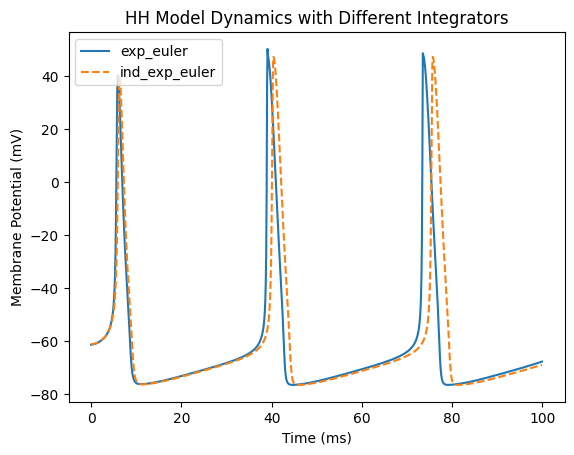
plt.title('HH Model Dynamics with Different Integrators')
plt.show()

Result Interpretation

After running the code, you will see the membrane potential over time.

Key conclusions: Action potential characteristics: Both methods can simulate the generation of action potentials, but the waveform details differ. Integrator differences:

• exp_euler produces smoother curves, fitting the relationship between tightly coupled gating variables and membrane potential more accurately, with action potential peaks and time courses closer to theoretical values.

• ind_exp_euler updates state variables independently, which may introduce slight deviations during rapid changes, but it is faster, especially for large-scale simulations. Applicable scenarios:

• For high-precision single-cell simulations, such as reproducing specific electrophysiological experiments, prefer exp_euler.

• For large-scale network simulations involving thousands of neurons, ind_exp_euler can significantly improve efficiency while maintaining sufficient accuracy.

Extended Exercises

• Try using the fourth-order Runge-Kutta method solver='rk4' and compare its accuracy and computational efficiency with exponential Euler methods.

• Adjust the input current intensity to observe how different integrators affect neuronal firing frequency.

• Extend the simulation duration to analyze the cumulative effect of integration errors over long-term simulations.

Through these exercises, you will gain a deeper understanding of the critical role of numerical methods in neural simulations and provide guidance for complex model design.

More

For more numerical integration methods, we provide a rich set of integrators and related resources in the Numerical Integration Methods Library.