Ions

In braincell, ions are divided into the following three base classes:

• Calcium: calcium ions

• Potassium: potassium ions

• Sodium: sodium ions

Using Existing Ions

First, let’s explain how to use the existing ions.

In practice, calling models related to these ions is very straightforward.

Ion Usage

Similarly, let’s look at an example of modeling an HH neuron:

import braincell

class HH(braincell.SingleCompartment):
    def __init__(self, in_size):
        super().__init__(in_size, C=Cm, solver='ind_exp_euler')
        self.na = braincell.ion.SodiumFixed(in_size, E=50. * u.mV)
        self.na.add_elem(
            INa=braincell.channel.INa_TM1991(in_size, g_max=(100. * u.mS * u.cm ** -2) * area, V_sh=-63. * u.mV)
        )

        self.k = braincell.ion.PotassiumFixed(in_size, E=-90 * u.mV)
        self.k.add_elem(
            IK=braincell.channel.IK_TM1991(in_size, g_max=(30. * u.mS * u.cm ** -2) * area, V_sh=-63. * u.mV)
        )

        self.IL = braincell.channel.IL(in_size, E=-60. * u.mV, g_max=(5. * u.nS * u.cm ** -2) * area)

First, after importing the relevant modules, we need to create specific model objects in the __init__ method.

Here, using sodium ion na as an example, we use SodiumDetailed to create a calcium ion model. We only need to set the parameters of SodiumDetailed according to definitions in the literature or the actual scenario.

As you can see, using pre-modeled ion models is very simple—just a straightforward call is enough.

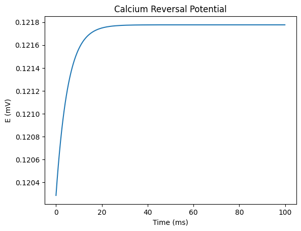
Similarly, we can perform simple simulations by calling a specific Ion type. For example, we can use CalciumDetailed to simulate the dynamic changes of intracellular calcium reversal potential over time.

import matplotlib.pyplot as plt
import brainstate
import braintools
import braincell
import brainunit as u

ca = braincell.ion.CalciumDetailed(size=1)
V = -65 * u.mV
ca.init_state(V)

dt = 0.1 * u.ms
steps = 1000

def run_calcium(i):
    t = i * dt
    with brainstate.environ.context(i=i, t=t, dt=dt):
        # Inward Currents
        input_current = -0.1 * u.uA / u.cm**2
        ca.C.derivative = input_current / (2 * u.faraday_constant * ca.d) + (ca.C_rest - ca.C.value) / ca.tau
        ca.C.value = ca.C.value + ca.C.derivative * dt
    return ca.E

indices = u.math.arange(steps)
E = brainstate.transform.for_loop(run_calcium, indices)

plt.plot(indices * dt, E)
plt.xlabel('Time (ms)')
plt.ylabel('E (mV)')
plt.title('Calcium Reversal Potential')
plt.show()

MixIons Usage

In some complex models, a single channel may involve the cooperative action of multiple ions. For example, certain calcium-activated potassium channels depend both on calcium concentration and membrane potential to regulate potassium efflux. Such multi-ion dependent mechanisms are very common in biological systems.

To address this, braincell provides a specialized module called MixIons for modeling composite channel systems driven by multiple ions.

MixIons inherits from IonChannel and Container, conforms to the channel component interface, and can host multiple submodules, making it convenient to manage multiple Channel objects. Similarly, MixIons supports the interfaces we discussed earlier.

In summary, MixIons provides a modular way to combine multiple Ion objects and multiple Channel objects, making it particularly suitable for channels that depend on multiple ion states or for integrating multiple channel currents in a model. With MixIons, you can build more flexible and precise neuronal dynamics models while maintaining clean and maintainable code structure.

Let’s look at an example of using MixIons in practical modeling:

class HTC(braincell.SingleCompartment):
    def __init__(
        self,
        size,
        gKL=0.01 * (u.mS / u.cm ** 2),
        V_initializer=braintools.init.Constant(-65. * u.mV),
        solver: str = 'ind_exp_euler'
    ):
        super().__init__(size, V_initializer=V_initializer, V_th=20. * u.mV, solver=solver)

        self.area = 1e-3 / (2.9e-4 * u.cm ** 2)

        self.k = braincell.ion.PotassiumFixed(size, E=-90. * u.mV)
        self.k.add(IKL=braincell.channel.IK_Leak(size, g_max=gKL))
        self.k.add(IDR=braincell.channel.IKDR_Ba2002(size, V_sh=-30. * u.mV, phi=0.25))

        self.ca = braincell.ion.CalciumDetailed(size, C_rest=5e-5 * u.mM, tau=10. * u.ms, d=0.5 * u.um)
        self.ca.add(ICaL=braincell.channel.ICaL_IS2008(size, g_max=0.5 * (u.mS / u.cm ** 2)))
        self.ca.add(ICaN=braincell.channel.ICaN_IS2008(size, g_max=0.5 * (u.mS / u.cm ** 2)))
        self.ca.add(ICaT=braincell.channel.ICaT_HM1992(size, g_max=2.1 * (u.mS / u.cm ** 2)))
        self.ca.add(ICaHT=braincell.channel.ICaHT_HM1992(size, g_max=3.0 * (u.mS / u.cm ** 2)))

        self.kca = braincell.MixIons(self.k, self.ca)
        self.kca.add(IAHP=braincell.channel.IAHP_De1994(size, g_max=0.3 * (u.mS / u.cm ** 2)))

In this example, other ions and their associated channels are omitted, and we focus on modeling the mixed ions.

If integration with other ions is needed, such as the kca mixed-ion example, you can simply use a mixed-ion pool with MixIons(self.k, self.ca).

Here, it is important to note that the order of ions passed in matters. For example:

braincell.channel.IAHP_De1994.root_type

JointTypes[braincell.ion.Potassium, braincell.ion.Calcium]

You can see that for a channel like IAHP_De1994, which involves multiple ions, the order of the two Ion types in its root_type matters. Thus, when passing ions to MixIons, the order must match exactly. For example, for IAHP_De1994, you must pass (self.k, self.ca) and not (self.ca, self.k) to avoid modeling errors caused by mismatched ion types.

In summary, as long as you have models for all the ions you want to integrate, like k and ca in this example, you can easily use MixIons to combine them.

---

Custom Ion Modeling

In practical modeling, the built-in ion types (Ca, K, Na) may not be sufficient. You might need to model other ions like Cl or require more detailed control over existing ions. Here, we will explain how to perform custom ion modeling.

Ion Modeling

From a physiological perspective, ions pass through the membrane selectively via channels. In programming, this dependency is reflected in the inheritance structure: Ion inherits from both IonChannel and Container. This means an Ion both provides channel interfaces and can contain multiple submodules.

In a simulation system, an Ion is attached to a HHTypedNeuron cell and, together with the membrane potential, drives the evolution of channels.

In braincell, Ion is an abstract entity for managing a specific type of ion. It does not directly produce current; instead, it organizes and orchestrates multiple Channel objects that carry the actual ionic currents. Each ion type corresponds to an Ion instance that acts as a container and control center for its associated channels, ensuring unified management.

Ion provides a set of simulation interfaces to manage its state evolution. Modeling ions this way allows for modular code structure and centralized management of all channels related to a particular ion. It also enables easy component reuse, improving efficiency.

During modeling, we often need to share key properties of ions, such as concentration and reversal potential, across multiple channels or functions. To handle this efficiently, braincell introduces a dedicated data structure: IonInfo.

IonInfo has two key attributes:

• C : Ion concentration

• E : Reversal potential

IonInfo acts as a lightweight container to manage and pass ion-related information, bridging Ion and Channel objects. It is a simple yet powerful mechanism for information flow in the simulation framework.

With this understanding, we are ready to model specific ions. Let’s take calcium as an example:

from typing import Union, Callable, Optional
from braincell.ion import Calcium

class CalciumFixed(Calcium):

    __module__ = 'braincell.ion'

    def __init__(
        self,
        size: brainstate.typing.Size,
        E: Union[brainstate.typing.ArrayLike, Callable] = 120. * u.mV,
        C: Union[brainstate.typing.ArrayLike, Callable] = 2.4e-4 * u.mM,
        name: Optional[str] = None,
        **channels
    ):
        super().__init__(size, name=name, **channels)
        self.E = braintools.init.param(E, self.varshape, allow_none=False)
        self.C = braintools.init.param(C, self.varshape, allow_none=False)

    def reset_state(self, V, batch_size=None):
        ca_info = self.pack_info()
        nodes = brainstate.graph.nodes(self, Channel, allowed_hierarchy=(1, 1)).values()
        self.check_hierarchies(type(self), *tuple(nodes))
        for node in nodes:
            node.reset_state(V, ca_info, batch_size=batch_size)

We can very easily model CalciumFixed, which inherits from Calcium and implements a general-purpose calcium ion model.

When modeling specific ions, you can follow the structure shown above. The most important part of defining a new ion is setting its key attributes, E (reversal potential) and C (concentration).

Based on this, you can create custom ion models for any ions you need in your simulations.

We continue using calcium as an example to further explain how to model more detailed dynamic ions, such as CalciumDetailed.

The modeling of CalciumDetailed is based on the model proposed by Bazhenov in 1998. In this model, calcium dynamics can be simplified as a first-order linear differential equation:

\[ \frac{d[Ca^{2+}]_i}{dt} = -\frac{I_{Ca}}{z F d} + \frac{[Ca^{2+}]_{\text{rest}} - [Ca^{2+}]_i}{\tau_{Ca}} \]

We implement this differential equation in braincell as follows:

from braincell.ion.calcium import _CalciumDynamics

class CalciumDetailed(_CalciumDynamics):

    __module__ = 'braincell.ion'

In this model, the parameters are as follows:

• \(I_{Ca}\): total calcium current produced by all calcium channels

• \(d\): thickness of the submembrane shell (\(1,\mu\mathrm{m}\))

• \(F\): Faraday constant

• \(\tau_{Ca}\): calcium removal time constant

• \([Ca^{2+}]_{\text{rest}} = 0.05,\mu\mathrm{M}\)

Based on these, we define the corresponding parameters:

    def __init__(
        self,
        size: brainstate.typing.Size,
        T: Union[brainstate.typing.ArrayLike, Callable] = u.celsius2kelvin(36.),
        d: Union[brainstate.typing.ArrayLike, Callable] = 1. * u.um,
        tau: Union[brainstate.typing.ArrayLike, Callable] = 5. * u.ms,
        C_rest: Union[brainstate.typing.ArrayLike, Callable] = 2.4e-4 * u.mM,
        C0: Union[brainstate.typing.ArrayLike, Callable] = 2. * u.mM,
        C_initializer: Union[brainstate.typing.ArrayLike, Callable] = braintools.init.Constant(2.4e-4 * u.mM),
        name: Optional[str] = None,
        **channels
    ):
        super().__init__(size, name=name, T=T, C0=C0, C_initializer=C_initializer, **channels)

        # parameters
        self.d = braintools.init.param(d, self.varshape, allow_none=False)
        self.tau = braintools.init.param(tau, self.varshape, allow_none=False)
        self.C_rest = braintools.init.param(C_rest, self.varshape, allow_none=False)

Then, according to the relevant formula:

\[ \frac{d[Ca^{2+}]_i}{dt} = -\frac{I_{Ca}}{z F d} + \frac{[Ca^{2+}]_{\text{rest}} - [Ca^{2+}]_i}{\tau_{Ca}} \]

where \(z = 2\), representing the valence of \(\mathrm{Ca^{2+}}\).

    def derivative(self, C, V):
        ICa = self.current(V, include_external=True)
        drive = ICa / (2 * u.faraday_constant * self.d)
        drive = u.math.maximum(drive, u.math.zeros_like(drive))
        return drive + (self.C_rest - C) / self.tau

At this point, we have completed the modeling of CalciumDetailed, implementing a classical dynamic calcium concentration model.

CalciumDetailed inherits from the _CalciumDynamics base class, which itself is a subclass of Calcium. Through this inheritance hierarchy, we can understand the recommended conventions for ion modeling.

In summary:

• For general-purpose ions, such as CalciumFixed, modeling requires defining the key properties E (reversal potential) and C (concentration).

• For more detailed ions, such as CalciumDetailed, modeling requires defining the dynamics according to the actual governing equations.

Through this tutorial, you have learned how to model new ions in braincell.

Existing Ion Instances

Our existing ion models are also quite rich. The following is an introduction to the relevant ions.

Calcium

In braincell, we extend the Ion class to model various specific types of ions. Here, we focus on the modeling approach for calcium ions (Calcium).

Calcium ions play a crucial role in neurons, participating in action potential initiation, neurotransmitter release, and various calcium-dependent signaling pathways. Therefore, for different modeling needs, we provide multiple versions of calcium ion models:

• CalciumFixed: calcium ion model with fixed concentration and reversal potential.

• CalciumDetailed: detailed calcium dynamics model based on biophysical mechanisms.

• CalciumFirstOrder: simplified first-order calcium dynamics model.

Before understanding these different models, we first explain the base class Calcium.

Calcium is the base class for all calcium ion models. It does not contain any specific dynamics itself and serves only as a semantic label, i.e., a calcium-specialized version of Ion, facilitating unified management and constraints for calcium ions.

CalciumFixed

CalciumFixed provides the simplest form of calcium modeling, assuming the calcium ion reversal potential E and concentration C are fixed and do not change over time.

CalciumDetailed

Intracellular Calcium Dynamics

The changes in intracellular calcium concentration are primarily determined by two mechanisms:

Influx through Calcium Currents

Calcium ions enter the cell through calcium channels and diffuse into the interior. The model only considers the submembrane shell region’s calcium concentration. The influx formula is:

\[ [Ca]_i = -\frac{I_{Ca}}{2 F d} \]

Where:

• \(F = 96489, \mathrm{C/mol}\) is Faraday’s constant

• \(d = 1, \mu\mathrm{m}\) is the thickness of the submembrane shell region

• \(I_{Ca}\) is the total current from all calcium channels

• \([Ca]_i\) is the intracellular calcium concentration

Efflux via Calcium Pumps

In the submembrane region, calcium removal occurs through binding to buffers, pump activity, diffusion, etc. Here, the model only considers pumps and uses the following kinetic reaction:

\[ \mathrm{Ca^{2+}_i} + P \underset{c_2}{\overset{c_1}{\rightleftharpoons}} \mathrm{CaP} \xrightarrow{c_3} P + \mathrm{Ca^{2+}_0} \]

Where:

• \(P\) represents the calcium pump

• \(\mathrm{CaP}\) is the intermediate complex in the pump

• \(\mathrm{Ca^{2+}_0}\) is the extracellular calcium concentration

• \(c_1\), \(c_2\), \(c_3\) are reaction rate constants

Considering \(c_3\) is very small, we can use the Michaelis-Menten approximation for the pump kinetics:

\[ \frac{d[Ca^{2+}]_i}{dt} = -\frac{K_T [Ca]_i}{[Ca]_i + K_d} \]

Where:

• \(K_T = 10^{-4}, \mathrm{mM/ms}\)

• \(K_d = \frac{c_2}{c_1} = 10^{-4}, \mathrm{mM}\)

• \(K_d\) is the calcium concentration at half-activation of the pump

Simplified First-Order Model

In the model proposed by Bazhenov in 1998, calcium dynamics can be simplified as a first-order linear differential equation:

\[ \frac{d[Ca^{2+}]_i}{dt} = -\frac{I_{Ca}}{z F d} + \frac{[Ca^{2+}]_{\text{rest}} - [Ca^{2+}]_i}{\tau_{Ca}} \]

Where:

• \(I_{Ca}\): total current from all calcium channels

• \(d\): thickness of the submembrane shell (1 μm)

• \(z = 2\): valence of \(\mathrm{Ca^{2+}}\)

• \(F\): Faraday’s constant

• \(\tau_{Ca}\): calcium clearance time constant

• \([Ca^{2+}]_{\text{rest}} = 0.05 \mu\mathrm{M}\)

Calcium Reversal Potential

The calcium reversal potential is given by the Nernst equation:

\[ E = \frac{RT}{2F} \log \left( \frac{[Ca^{2+}]_0}{[Ca^{2+}]_i} \right) \]

Where:

• \(R = 8.31441, \mathrm{J/(mol\cdot K)}\): gas constant

• \(T = 309.15, \mathrm{K}\): absolute temperature (~36℃)

• \(F = 96489, \mathrm{C/mol}\): Faraday’s constant

• \([Ca^{2+}]_0 = 2, \mathrm{mM}\): extracellular calcium concentration

CalciumFirstOrder

This model uses a simple first-order differential equation to simulate calcium concentration changes:

\[ Ca' = -\alpha I_{Ca} + -\beta Ca \]

At this point, we have fully understood the several built-in calcium ion models in Calcium.

Potassium

For Potassium, we still extend the Ion class for modeling.

Potassium ions are widely present in neurons, and their transmembrane flow is crucial for maintaining the resting membrane potential, repolarization of action potentials, and controlling neuronal excitability.

Potassium is the base class for all potassium ion models. It inherits from Ion and is used for unified identification and organization of potassium ions. The class itself does not contain specific dynamics and serves only as an interface template. This class is mainly for structural and organizational purposes.

If actual modeling is needed, we use PotassiumFixed.

PotassiumFixed

PotassiumFixed provides the most basic potassium modeling approach, assuming its concentration and reversal potential are fixed and do not change over time. This model is suitable for situations where intracellular potassium dynamics are not of interest, only the potassium current and constant reversal potential are needed.

In reset_state, it packages E and C into an IonInfo object and passes it to all attached Channel submodules for subsequent current calculations.

Sodium

Similar to other ion models, sodium ions in braincell are modeled by extending the Ion class.

Sodium ions are core participants in action potential generation. Their inward flow leads to depolarization, which is a key mechanism for neuronal excitability and signal transmission.

Sodium is the abstract base class for all sodium ion models. It inherits from Ion and is used to uniformly manage sodium ion instances and provide a consistent structural interface. The class itself does not implement any dynamics and serves only as an interface template.

SodiumFixed

SodiumFixed provides the simplest form of sodium modeling, assuming its concentration C and reversal potential E are fixed and do not change over time.

This model is suitable for scenarios where only the magnitude of the sodium current is considered, and the time-dependent dynamics of sodium concentration are not required, commonly used in traditional Hodgkin-Huxley-type modeling.

Similarly, in the reset_state method, the model packages its reversal potential E and concentration C into an IonInfo object and propagates it to all bound Channel submodules for current calculation.