
Cell#
The core components of Cell include the following three parts:
HHTypeNeuron: The base class that provides the interface for HH-type neurons.SingleCompartment: A single-compartment neuron model, suitable for neurons with simple structures.MultiCompartment: A multi-compartment neuron model, suitable for neurons where spatial structure needs to be considered.
Together, these three components form a modeling system that spans from local membrane regions to the complete neuronal structure. Through inheritance, they share a unified modeling interface and, with the acceleration and computational power of brainstate, provide strong support for neuronal modeling at the cellular level.
HHTypedNeuron#
Electrophysiological Properties#
HHTypedNeuron is a fundamental abstract class in braincell for constructing Hodgkin–Huxley-type neuron models. In this modeling framework, the membrane potential of a neuron is determined by multiple currents:
Active currents: Controlled by sodium and potassium channels with voltage-gated properties.
Passive currents: Such as leak currents.
Capacitive currents: Arising from changes in membrane potential.
This modeling approach was first proposed by Hodgkin and Huxley in 1952 to explain the mechanism of action potentials in the squid giant axon. The HH model not only laid the foundation of modern neuronal modeling but also remains a core component of many models today.
The equivalent circuit diagram of the classical HH model is shown below:
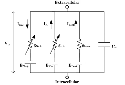
In the classical HH model, the membrane potential \(V\) is governed by the following equation:
Where:
\(C_m\): Membrane capacitance
\(I_{\text{Na}}, I_{\text{K}}\): Ionic currents from sodium and potassium channels
\(I_L\): Leak current
\(I_{\text{ext}}\): External injected current (e.g., current applied through a stimulating electrode)
Modeling Implementation#
HHTypedNeuron inherits from:
Dynamics: For defining state variables and differential equations.Container: For managing modules.DiffEqModule: A differential equation module that supports automatic modeling.
With HHTypedNeuron, you can flexibly combine ion channels to construct diverse dynamical configurations.
Moreover, since HHTypedNeuron is deeply integrated with brainstate, it also supports automatic differentiation and vectorized simulations, enabling batch simulations and model training.
Notably, in braincell, all neuron models are built upon the HH framework.
Specifically, both SingleCompartment and MultiCompartment inherit from HHTypedNeuron, sharing a unified interface and modeling framework. This allows us to reuse the same ion channel mechanisms and dynamical modeling strategies across neurons with different structural complexities.
SingleCompartment#
Electrophysiological Properties#
SingleCompartment represents a neuron model without explicit spatial structure, used for modeling conductance-based neurons with a single compartment. Its membrane potential is governed by the following differential equation:
Where:
\(C_m\): Membrane capacitance
\(V\): Membrane potential
\(g_j\): Conductance of the \(j\)-th ion channel
\(E_j\): Reversal potential of the \(j\)-th channel
\(I_{\text{ext}}\): External injected current
The conductance \(g_j\) of each channel is determined by its gating variables:
Where:
\(\bar{g}_j\): Maximum conductance
\(M\): Activation variable
\(N\): Inactivation variable
\(x, y\): Exponents depending on channel type
The gating variables follow first-order kinetics:
Or equivalently:
Where:
\(x \in \{M, N\}\)
\(\phi_x\): Temperature factor
\(x_\infty\): Steady-state value
\(\tau_x\): Time constant
\(\alpha_x\), \(\beta_x\): Rate constants
Modeling Implementation#
The implementation of SingleCompartment is relatively straightforward: simply inherit from HHTypedNeuron and define the corresponding ion channels.
Here is an example:
class HH(braincell.SingleCompartment):
    def __init__(self, size, solver='rk4'):
        super().__init__(size, solver=solver)

        self.na = braincell.ion.SodiumFixed(size, E=50. * u.mV)
        self.na.add(INa=braincell.channel.INa_HH1952(size))

        self.k = braincell.ion.PotassiumFixed(size, E=-77. * u.mV)
        self.k.add(IK=braincell.channel.IK_HH1952(size))

        self.IL = braincell.channel.IL(
            size,
            E=-54.387 * u.mV,
            g_max=0.03 * (u.mS / u.cm **2)
        )
In this example, we use SingleCompartment to construct a classical HH neuron with sodium (INa), potassium (IK), and leak (IL) currents, which together determine the electrophysiological properties of the neuron.
As this example shows, SingleCompartment serves as a convenient modeling interface in braincell, greatly simplifying the construction of neurons and improving modeling efficiency.
MultiCompartment#
Electrophysiological Properties#
In real neurons, the cell is not just a point-like structure but instead has complex spatial morphology—dendrites, axons, and soma—all of which strongly influence neuronal behavior. To simulate spatial propagation of electrical signals more accurately, we introduce MultiCompartment.
A neuron is not simply a capacitor but behaves as a cable-like system with spatial structure. Cable theory describes how electrical signals propagate along thin neuronal processes such as dendrites or axons. Originating from engineering transmission line theory, in neuroscience it treats dendrites and axons as one-dimensional cables, allowing us to simulate spatiotemporal variations in signals.
In computational models, cable theory is typically implemented through compartmental modeling: the neuron is divided into discrete compartments, each represented as an equivalent circuit unit. Neighboring compartments are coupled by axial resistances, approximating the spatial structure.
This is precisely the core principle of MultiCompartment modeling.
In this approach, the neuron is divided into multiple spatially connected compartments, each with independent membrane potentials and ionic currents, while being coupled via axial resistances:
Each compartment has its own distribution of ion channels and currents.
Compartments are interconnected via resistances that allow axial current flow.
This enables modeling of phenomena such as attenuation, delay, or reflection of signals along dendrites or axons.
The schematic of cable theory is shown below:
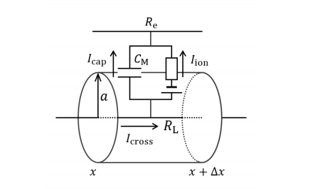
The electrical behavior is governed by the cable equation:
Where:
\(C_m\): Membrane capacitance
\(I_{\text{ion}, i}\): Ionic current in the \(i\)-th compartment
\(\frac{(V_j - V_i)}{R_{ij}}\): Axial current flowing from neighboring compartment \(j\) to \(i\)
\(R_{ij}\): Axial resistance between compartments \(i\) and \(j\)
\(I_{\text{ext}, i}\): External injected current into compartment \(i\)
Thanks to its spatial modeling capabilities, the multi-compartment model is widely used to study dendritic integration, action potential propagation along axons, and other spatially dependent phenomena.
Modeling Implementation#
The implementation of MultiCompartment is conceptually similar to SingleCompartment, but requires specifying additional parameters, most importantly the morphology.
Here is an example:
class HTC(braincell.MultiCompartment):
    def __init__(self, size, solver: str = 'staggered'):
        morphology = braincell.Morphology.from_swc(...)
        super().__init__(size,
                         morphology=morphology,   # the only difference from SingleCompartment
                         V_initializer=braintools.init.Constant(-65. * u.mV),
                         V_th=20. * u.mV,
                         solver=solver)

        self.na = braincell.ion.SodiumFixed(size, E=50. * u.mV)
        self.na.add(INa=braincell.channel.INa_Ba2002(size, V_sh=-30 * u.mV))

        self.k = braincell.ion.PotassiumFixed(size, E=-90. * u.mV)
        self.k.add(IDR=braincell.channel.IKDR_Ba2002(size, V_sh=-30. * u.mV, phi=0.25))
This example demonstrates how to construct a simple multi-compartment neuron model with sodium and potassium channels. Of course, the model can be extended further by adding additional channels or input currents.
The critical difference between SingleCompartment and MultiCompartment lies in the introduction of morphology.
In neuronal modeling, morphology refers to the spatial structure of the neuron, including:
Soma
Dendrites
Axon
Spatial connectivity
In short:
In
SingleCompartment, the neuron is modeled as a point.In
MultiCompartment, the neuron is modeled as a network of compartments defined by its morphology, allowing more realistic dynamical simulations.
Through MultiCompartment, we can easily construct neuron models with detailed structures and diverse behaviors.