Functional API and Graph Operations

This tutorial demonstrates how to use BrainState’s functional API for explicit state management using graph operations. This approach provides fine-grained control over model states and is particularly useful for advanced use cases like custom training loops and functional transformations.

Learning Objectives

By the end of this tutorial, you will:

• Understand the functional API and graph operations in BrainState

• Learn how to split and merge model states using treefy_split and treefy_merge

• Build a training loop with explicit state management

• Apply JAX transformations with separated states

• Track custom states (e.g., function call counts)

Setup and Imports

First, let’s import the necessary libraries:

import jax
import jax.numpy as jnp
import matplotlib.pyplot as plt
import numpy as np

import brainstate

# Set random seed for reproducibility
np.random.seed(42)

Problem: Polynomial Regression

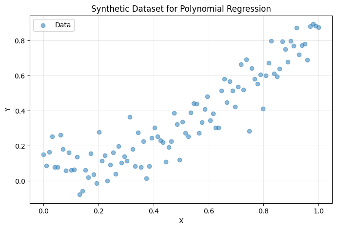
We’ll solve a simple polynomial regression problem to demonstrate the functional API. Let’s create a synthetic dataset:

# Generate synthetic data: y = 0.8 * x^2 + 0.1 + noise
X = np.linspace(0, 1, 100)[:, None]
Y = 0.8 * X ** 2 + 0.1 + np.random.normal(0, 0.1, size=X.shape)

def dataset(batch_size):
    """Generator that yields random batches from the dataset."""
    while True:
        idx = np.random.choice(len(X), size=batch_size)
        yield X[idx], Y[idx]

# Visualize the data
plt.figure(figsize=(8, 5))
plt.scatter(X, Y, alpha=0.5, label='Data')
plt.xlabel('X')
plt.ylabel('Y')
plt.title('Synthetic Dataset for Polynomial Regression')
plt.legend()
plt.grid(True, alpha=0.3)
plt.show()

Building the Model

Step 1: Define Basic Components

First, let’s create a simple Linear layer and a custom state type to track function calls:

class Linear(brainstate.nn.Module):
    """A simple linear layer: y = x @ w + b"""
    
    def __init__(self, din: int, dout: int):
        super().__init__()
        # Initialize weights and biases as trainable parameters
        self.w = brainstate.ParamState(brainstate.random.rand(din, dout))
        self.b = brainstate.ParamState(jnp.zeros((dout,)))
    
    def __call__(self, x):
        return x @ self.w.value + self.b.value


class Count(brainstate.State):
    """Custom state type for tracking function calls."""
    pass

Step 2: Build the MLP Model

Now let’s create a multi-layer perceptron (MLP) with a call counter:

class MLP(brainstate.graph.Node):
    """Multi-layer perceptron with call counting."""
    
    def __init__(self, din, dhidden, dout):
        # Custom state to count how many times the model is called
        self.count = Count(jnp.array(0))
        
        # Two linear layers
        self.linear1 = Linear(din, dhidden)
        self.linear2 = Linear(dhidden, dout)
    
    def __call__(self, x):
        # Increment call counter
        self.count.value += 1
        
        # Forward pass
        x = self.linear1(x)
        x = jax.nn.relu(x)
        x = self.linear2(x)
        return x

Understanding Graph Operations

What are Graph Operations?

BrainState models are represented as computational graphs where:

• Nodes represent modules or components

• States are the mutable variables within these nodes

Graph operations allow you to:

1. Split a model into its graph definition and separate state pytrees

2. Merge a graph definition with state pytrees to reconstruct the model

This is essential for functional programming with JAX, as it allows you to:

• Pass states as explicit function arguments

• Apply JAX transformations (jit, grad, vmap) to functions operating on states

• Manage different types of states independently (e.g., parameters vs. counters)

Splitting the Model

Let’s create a model and split it into its components:

# Create the model
model_initial = MLP(din=1, dhidden=32, dout=1)

# Split the model into graph definition and states
graphdef, params_, counts_ = brainstate.graph.treefy_split(
    model_initial, 
    brainstate.ParamState,  # Split out trainable parameters
    Count                    # Split out call counters
)

print("Graph definition (model structure):")
print(graphdef)
print("\nParameters (trainable weights):")
print(jax.tree.map(jnp.shape, params_))
print("\nCounters:")
print(counts_)

Graph definition (model structure):
NodeDef(
  type=MLP,
  index=0,
  attributes=('count', 'linear1', 'linear2'),
  subgraphs={
    'linear1': NodeDef(
      type=Linear,
      index=2,
      attributes=('_in_size', '_name', '_out_size', 'b', 'w'),
      subgraphs={
        '_in_size': NodeDef(
          type=PytreeType,
          index=-1,
          attributes=(),
          subgraphs={},
          static_fields={},
          leaves={},
          metadata=PyTreeDef(None),
          index_mapping=None
        ),
        '_name': NodeDef(
          type=PytreeType,
          index=-1,
          attributes=(),
          subgraphs={},
          static_fields={},
          leaves={},
          metadata=PyTreeDef(None),
          index_mapping=None
        ),
        '_out_size': NodeDef(
          type=PytreeType,
          index=-1,
          attributes=(),
          subgraphs={},
          static_fields={},
          leaves={},
          metadata=PyTreeDef(None),
          index_mapping=None
        )
      },
      static_fields={},
      leaves={
        'b': NodeRef(
          type=ParamState,
          index=3
        ),
        'w': NodeRef(
          type=ParamState,
          index=4
        )
      },
      metadata=(<class '__main__.Linear'>,),
      index_mapping=None
    ),
    'linear2': NodeDef(
      type=Linear,
      index=5,
      attributes=('_in_size', '_name', '_out_size', 'b', 'w'),
      subgraphs={
        '_in_size': NodeDef(
          type=PytreeType,
          index=-1,
          attributes=(),
          subgraphs={},
          static_fields={},
          leaves={},
          metadata=PyTreeDef(None),
          index_mapping=None
        ),
        '_name': NodeDef(
          type=PytreeType,
          index=-1,
          attributes=(),
          subgraphs={},
          static_fields={},
          leaves={},
          metadata=PyTreeDef(None),
          index_mapping=None
        ),
        '_out_size': NodeDef(
          type=PytreeType,
          index=-1,
          attributes=(),
          subgraphs={},
          static_fields={},
          leaves={},
          metadata=PyTreeDef(None),
          index_mapping=None
        )
      },
      static_fields={},
      leaves={
        'b': NodeRef(
          type=ParamState,
          index=6
        ),
        'w': NodeRef(
          type=ParamState,
          index=7
        )
      },
      metadata=(<class '__main__.Linear'>,),
      index_mapping=None
    )
  },
  static_fields={},
  leaves={
    'count': NodeRef(
      type=Count,
      index=1
    )
  },
  metadata=(<class '__main__.MLP'>,),
  index_mapping=None
)

Parameters (trainable weights):
{
  'linear1': {
    'b': TreefyState(
      type=<class 'brainstate.ParamState'>,
      value=(32,),
      tag=None
    ),
    'w': TreefyState(
      type=<class 'brainstate.ParamState'>,
      value=(1, 32),
      tag=None
    )
  },
  'linear2': {
    'b': TreefyState(
      type=<class 'brainstate.ParamState'>,
      value=(1,),
      tag=None
    ),
    'w': TreefyState(
      type=<class 'brainstate.ParamState'>,
      value=(32, 1),
      tag=None
    )
  }
}

Counters:
{
  'count': TreefyState(
    type=<class '__main__.Count'>,
    value=Array(0, dtype=int32, weak_type=True),
    tag=None
  )
}

Key Points:

• graphdef: Contains the model structure (immutable)

• params_: PyTree of trainable parameters (ParamState)

• counts_: PyTree of counters (Count state)

This separation is crucial because:

1. Only params_ needs gradients during training

2. counts_ needs to be updated but not differentiated

3. graphdef remains constant throughout training

Functional Training Loop

Step 1: Define Training Step

With separated states, we can create a pure functional training step:

@jax.jit
def train_step(params, counts, batch):
    """Perform one training step with explicit state management."""
    x, y = batch
    
    def loss_fn(params):
        # Merge graph definition with states to reconstruct the model
        model = brainstate.graph.treefy_merge(graphdef, params, counts)
        
        # Forward pass
        y_pred = model(x)
        
        # Extract updated counters (model was called, so count changed)
        new_counts = brainstate.graph.treefy_states(model, Count)
        
        # Compute loss
        loss = jnp.mean((y - y_pred) ** 2)
        
        return loss, new_counts
    
    # Compute gradients with respect to parameters
    grad, counts = jax.grad(loss_fn, has_aux=True)(params)
    
    # Simple SGD update: params = params - lr * grad
    params = jax.tree.map(lambda w, g: w - 0.1 * g, params, grad)
    
    return params, counts

Understanding the Training Step:

1. Loss Function Definition:

   • Takes params as input (what we differentiate)

   • Merges graphdef, params, and counts to reconstruct the model

   • Computes predictions and loss

   • Returns both loss and updated counts (auxiliary output)

2. Gradient Computation:

   • jax.grad computes gradients of loss w.r.t. parameters

   • has_aux=True allows returning both gradients and auxiliary values (counts)

3. Parameter Update:

   • Simple gradient descent: new_params = old_params - learning_rate * gradients

   • Uses jax.tree.map to apply the update to all parameters in the pytree

Step 2: Define Evaluation Step

@jax.jit
def eval_step(params, counts, batch):
    """Evaluate the model on a batch."""
    x, y = batch
    
    # Reconstruct model
    model = brainstate.graph.treefy_merge(graphdef, params, counts)
    
    # Forward pass
    y_pred = model(x)
    
    # Compute loss
    loss = jnp.mean((y - y_pred) ** 2)
    
    return {'loss': loss}

Step 3: Run Training

# Training parameters
total_steps = 10_000

# Training loop
print("Training the model...\n")
for step, batch in enumerate(dataset(32)):
    # Update parameters and counters
    params_, counts_ = train_step(params_, counts_, batch)
    
    # Log progress every 1000 steps
    if step % 1000 == 0:
        logs = eval_step(params_, counts_, (X, Y))
        print(f"Step: {step:5d}, Loss: {logs['loss']:.6f}")
    
    # Stop after total_steps
    if step >= total_steps - 1:
        break

print("\nTraining complete!")

Training the model...

Step:     0, Loss: 2.924491
Step:  1000, Loss: 0.007898
Step:  2000, Loss: 0.007857
Step:  3000, Loss: 0.007903
Step:  4000, Loss: 0.007962
Step:  5000, Loss: 0.007840
Step:  6000, Loss: 0.007831
Step:  7000, Loss: 0.007867
Step:  8000, Loss: 0.007872
Step:  9000, Loss: 0.007837

Training complete!

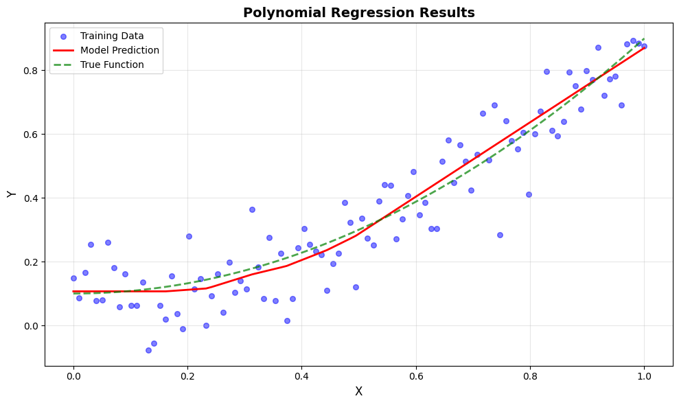
Analyzing Results

Reconstruct the Final Model

After training, we can merge the learned parameters back into a model:

# Reconstruct the trained model
model = brainstate.graph.treefy_merge(graphdef, params_, counts_)

# Check how many times the model was called during training
print(f"Total model calls during training: {model.count.value}")

# Make predictions on the full dataset
y_pred = model(X)

print(f"Final predictions shape: {y_pred.shape}")

Total model calls during training: 10000
Final predictions shape: (100, 1)

Visualize Predictions

plt.figure(figsize=(10, 6))

# Plot data points
plt.scatter(X, Y, color='blue', alpha=0.5, label='Training Data', s=30)

# Plot predictions
plt.plot(X, y_pred, color='red', linewidth=2, label='Model Prediction')

# Plot true function
X_true = np.linspace(0, 1, 100)[:, None]
Y_true = 0.8 * X_true ** 2 + 0.1
plt.plot(X_true, Y_true, color='green', linewidth=2, 
         linestyle='--', label='True Function', alpha=0.7)

plt.xlabel('X', fontsize=12)
plt.ylabel('Y', fontsize=12)
plt.title('Polynomial Regression Results', fontsize=14, fontweight='bold')
plt.legend(fontsize=10)
plt.grid(True, alpha=0.3)
plt.tight_layout()
plt.show()

Key Concepts Summary

Graph Operations

1. treefy_split(model, *state_types):

   • Splits a model into graph definition and state pytrees

   • Returns: (graphdef, state1, state2, ...)

   • Allows independent management of different state types

2. treefy_merge(graphdef, *states):

   • Reconstructs a model from graph definition and states

   • Returns: Complete model with all states

   • Essential for functional API usage

3. treefy_states(model, state_type):

   • Extracts states of a specific type from a model

   • Useful for getting updated states after forward pass

Advantages of Functional API

1. Explicit State Management: Full control over which states are updated and how

2. JAX Compatibility: States are explicit function arguments, making JAX transformations straightforward

3. Flexibility: Separate handling of parameters, hidden states, and custom states

4. Debugging: Easier to track state changes and debug issues

When to Use Functional API

• Custom training loops with complex state management

• Implementing advanced optimization algorithms

• Fine-grained control over gradient computation

• Functional programming style with JAX transformations

• Distributed training scenarios

Exercises

Try these exercises to deepen your understanding:

1. Add Momentum to SGD:

   • Create a custom state type for momentum

   • Modify the training step to include momentum updates

2. Track More Statistics:

   • Add states to track training loss history

   • Add states to track gradient norms

3. Implement Learning Rate Scheduling:

   • Create a state for the current learning rate

   • Implement exponential decay or step decay

4. Multi-Task Learning:

   • Modify the MLP to have multiple output heads

   • Track separate counters for each task

Next Steps

Now that you understand the functional API and graph operations, you can:

1. Explore Lifted Transforms: Learn about higher-level state management with automatic lifting

2. Advanced Optimizers: Use BrainTools optimizers that handle state management for you

3. Complex Architectures: Apply these concepts to recurrent networks and spiking neural networks

4. Checkpointing: Learn how to save and load model states

References

• BrainState Graph API Documentation

• JAX Transformations

• Flax Functional API