
Activation Functions and Normalization#
Activation functions and normalization layers are critical components that enable deep neural networks to learn complex patterns and train stably.
In this tutorial, you will learn:
🎯 Activation Functions - ReLU, GELU, Sigmoid, Tanh and variants
📊 Batch Normalization - Stabilizing training with BatchNorm
📐 Layer Normalization - Alternative normalization for sequences
🔲 Group Normalization - For small batch sizes
⚖️ When to use each - Practical guidelines
Why Are These Important?#
Activation Functions introduce non-linearity, allowing networks to learn complex patterns
Normalization Layers stabilize training, accelerate convergence, and act as regularizers
import brainstate
import jax.numpy as jnp
import matplotlib.pyplot as plt
import numpy as np
1. Activation Functions#
Activation functions determine the output of a neuron given its input.
ReLU Family#
Standard ReLU#
# ReLU: max(0, x)
relu = brainstate.nn.ReLU()

x = jnp.linspace(-3, 3, 100)
y = relu(x)

plt.figure(figsize=(10, 4))
plt.subplot(1, 2, 1)
plt.plot(x, y, linewidth=2, label='ReLU')
plt.axhline(0, color='gray', linestyle='--', alpha=0.3)
plt.axvline(0, color='gray', linestyle='--', alpha=0.3)
plt.grid(alpha=0.3)
plt.xlabel('Input')
plt.ylabel('Output')
plt.title('ReLU Activation', fontweight='bold')
plt.legend()

# Test with data
test_input = jnp.array([-2, -1, 0, 1, 2])
test_output = relu(test_input)
plt.subplot(1, 2, 2)
plt.stem(test_input, test_output, basefmt=' ')
plt.xlabel('Input')
plt.ylabel('Output')
plt.title('ReLU on Sample Points', fontweight='bold')
plt.grid(alpha=0.3)

plt.tight_layout()
plt.show()

print(f"Input:  {test_input}")
print(f"Output: {test_output}")
print("\n✅ Advantages: Simple, fast, no gradient vanishing for positive values")
print("⚠️  Issue: 'Dying ReLU' problem when neurons always output 0")
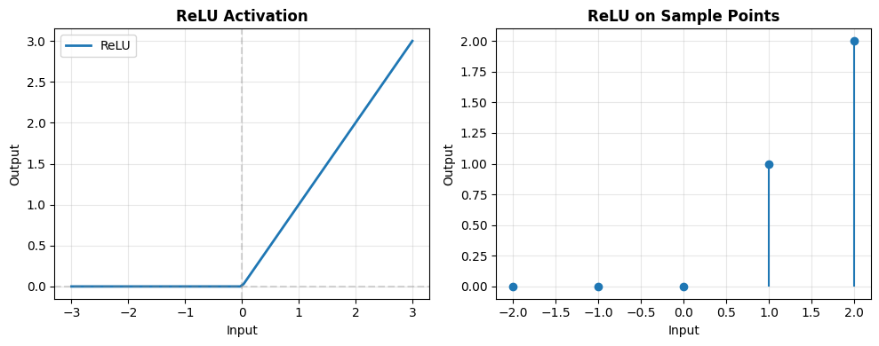
Input:  [-2 -1  0  1  2]
Output: [0 0 0 1 2]

✅ Advantages: Simple, fast, no gradient vanishing for positive values
⚠️  Issue: 'Dying ReLU' problem when neurons always output 0
Leaky ReLU#
# LeakyReLU: max(alpha * x, x)
leaky_relu = brainstate.nn.LeakyReLU(negative_slope=0.1)

y_leaky = leaky_relu(x)

plt.figure(figsize=(8, 5))
plt.plot(x, y, linewidth=2, label='ReLU', alpha=0.5)
plt.plot(x, y_leaky, linewidth=2, label='Leaky ReLU (α=0.1)')
plt.axhline(0, color='gray', linestyle='--', alpha=0.3)
plt.axvline(0, color='gray', linestyle='--', alpha=0.3)
plt.grid(alpha=0.3)
plt.xlabel('Input')
plt.ylabel('Output')
plt.title('ReLU vs Leaky ReLU', fontweight='bold')
plt.legend()
plt.show()

print("✅ Advantage: Allows small gradient for negative values")
print("   Helps prevent dying ReLU problem")
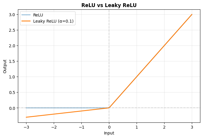
✅ Advantage: Allows small gradient for negative values
   Helps prevent dying ReLU problem
Modern Activation Functions#
GELU (Gaussian Error Linear Unit)#
# GELU: Smooth, probabilistic activation
gelu = brainstate.nn.GELU()

y_gelu = gelu(x)

plt.figure(figsize=(8, 5))
plt.plot(x, y, linewidth=2, label='ReLU', alpha=0.5)
plt.plot(x, y_gelu, linewidth=2, label='GELU')
plt.axhline(0, color='gray', linestyle='--', alpha=0.3)
plt.axvline(0, color='gray', linestyle='--', alpha=0.3)
plt.grid(alpha=0.3)
plt.xlabel('Input')
plt.ylabel('Output')
plt.title('ReLU vs GELU', fontweight='bold')
plt.legend()
plt.show()

print("✅ Used in Transformers (BERT, GPT)")
print("✅ Smooth, differentiable everywhere")
print("✅ Stochastic regularization properties")
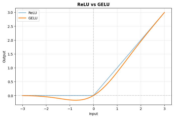
✅ Used in Transformers (BERT, GPT)
✅ Smooth, differentiable everywhere
✅ Stochastic regularization properties
Classic Activations#
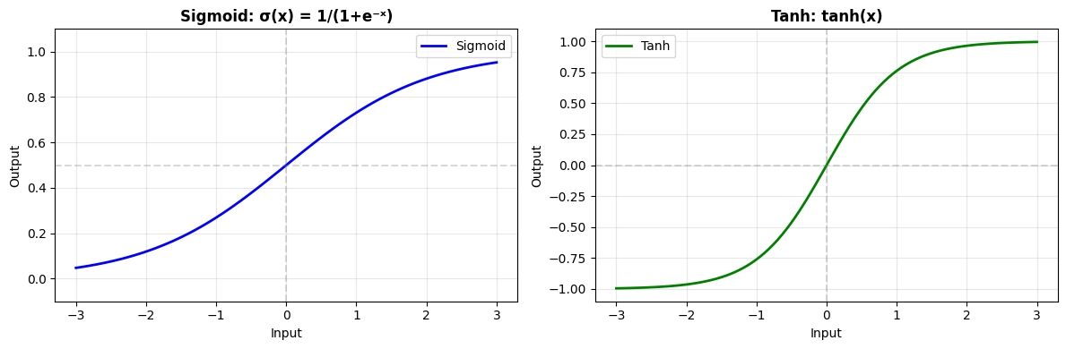
Sigmoid and Tanh#
# Sigmoid: 1 / (1 + exp(-x))
sigmoid = brainstate.nn.Sigmoid()

# Tanh: (exp(x) - exp(-x)) / (exp(x) + exp(-x))
tanh = brainstate.nn.Tanh()

y_sigmoid = sigmoid(x)
y_tanh = tanh(x)

plt.figure(figsize=(12, 4))

plt.subplot(1, 2, 1)
plt.plot(x, y_sigmoid, linewidth=2, label='Sigmoid', color='blue')
plt.axhline(0.5, color='gray', linestyle='--', alpha=0.3)
plt.axvline(0, color='gray', linestyle='--', alpha=0.3)
plt.grid(alpha=0.3)
plt.xlabel('Input')
plt.ylabel('Output')
plt.title('Sigmoid: σ(x) = 1/(1+e⁻ˣ)', fontweight='bold')
plt.legend()
plt.ylim([-0.1, 1.1])

plt.subplot(1, 2, 2)
plt.plot(x, y_tanh, linewidth=2, label='Tanh', color='green')
plt.axhline(0, color='gray', linestyle='--', alpha=0.3)
plt.axvline(0, color='gray', linestyle='--', alpha=0.3)
plt.grid(alpha=0.3)
plt.xlabel('Input')
plt.ylabel('Output')
plt.title('Tanh: tanh(x)', fontweight='bold')
plt.legend()
plt.ylim([-1.1, 1.1])

plt.tight_layout()
plt.show()

print("Sigmoid:")
print("  ✅ Output range: (0, 1) - good for probabilities")
print("  ⚠️  Vanishing gradients for large |x|")
print("\nTanh:")
print("  ✅ Output range: (-1, 1) - zero-centered")
print("  ⚠️  Also suffers from vanishing gradients")
print("  📝 Often used in RNN/LSTM gates")
Sigmoid:
  ✅ Output range: (0, 1) - good for probabilities
  ⚠️  Vanishing gradients for large |x|

Tanh:
  ✅ Output range: (-1, 1) - zero-centered
  ⚠️  Also suffers from vanishing gradients
  📝 Often used in RNN/LSTM gates
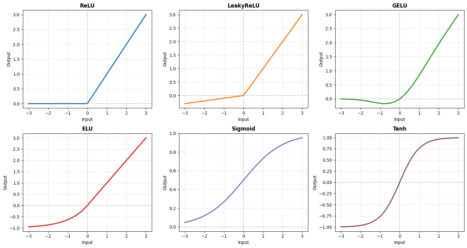
Comparing All Activations#
# Compare multiple activations
activations = {
    'ReLU': brainstate.nn.ReLU(),
    'LeakyReLU': brainstate.nn.LeakyReLU(0.1),
    'GELU': brainstate.nn.GELU(),
    'ELU': brainstate.nn.ELU(),
    'Sigmoid': brainstate.nn.Sigmoid(),
    'Tanh': brainstate.nn.Tanh(),
}

fig, axes = plt.subplots(2, 3, figsize=(15, 8))
axes = axes.flatten()

for idx, (name, activation) in enumerate(activations.items()):
    y_act = activation(x)
    axes[idx].plot(x, y_act, linewidth=2.5, color=f'C{idx}')
    axes[idx].axhline(0, color='gray', linestyle='--', alpha=0.3)
    axes[idx].axvline(0, color='gray', linestyle='--', alpha=0.3)
    axes[idx].grid(alpha=0.3)
    axes[idx].set_xlabel('Input', fontsize=10)
    axes[idx].set_ylabel('Output', fontsize=10)
    axes[idx].set_title(name, fontsize=12, fontweight='bold')

plt.tight_layout()
plt.show()

print("\n📊 Activation Function Guide:\n")
print("ReLU:        Default choice, fast, works well in most cases")
print("LeakyReLU:   When dying ReLU is a problem")
print("GELU:        Transformers, NLP models")
print("ELU:         Smooth variant of ReLU with negative values")
print("Sigmoid:     Output layer for binary classification")
print("Tanh:        RNN/LSTM gates, when zero-centered output needed")
📊 Activation Function Guide:

ReLU:        Default choice, fast, works well in most cases
LeakyReLU:   When dying ReLU is a problem
GELU:        Transformers, NLP models
ELU:         Smooth variant of ReLU with negative values
Sigmoid:     Output layer for binary classification
Tanh:        RNN/LSTM gates, when zero-centered output needed
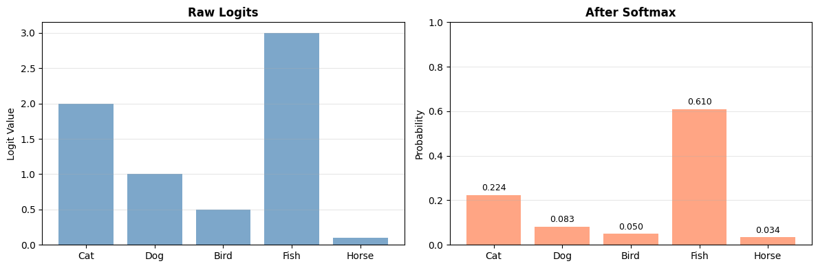
Softmax - For Classification#
# Softmax: converts logits to probabilities
softmax = brainstate.nn.Softmax()

# Example logits from a classifier
logits = jnp.array([2.0, 1.0, 0.5, 3.0, 0.1])
probs = softmax(logits)

print("Logits:       ", logits)
print("Probabilities:", probs)
print(f"Sum of probs:  {jnp.sum(probs):.6f} (should be 1.0)")

# Visualize
fig, axes = plt.subplots(1, 2, figsize=(12, 4))

classes = ['Cat', 'Dog', 'Bird', 'Fish', 'Horse']

axes[0].bar(classes, logits, color='steelblue', alpha=0.7)
axes[0].set_ylabel('Logit Value')
axes[0].set_title('Raw Logits', fontweight='bold')
axes[0].grid(axis='y', alpha=0.3)

axes[1].bar(classes, probs, color='coral', alpha=0.7)
axes[1].set_ylabel('Probability')
axes[1].set_title('After Softmax', fontweight='bold')
axes[1].set_ylim([0, 1])
axes[1].grid(axis='y', alpha=0.3)

# Add values on bars
for i, v in enumerate(probs):
    axes[1].text(i, v + 0.02, f'{v:.3f}', ha='center', fontsize=9)

plt.tight_layout()
plt.show()

print("\n✅ Softmax converts logits to valid probability distribution")
print("   Use for multi-class classification output layer")
Logits:        [2.  1.  0.5 3.  0.1]
Probabilities: [0.22427258 0.08250527 0.05004197 0.60963607 0.03354414]
Sum of probs:  1.000000 (should be 1.0)
✅ Softmax converts logits to valid probability distribution
   Use for multi-class classification output layer
2. Normalization Layers#
Normalization stabilizes training by controlling the distribution of activations.
Batch Normalization#
# BatchNorm: Normalizes across batch dimension
brainstate.random.seed(42)
batch_norm = brainstate.nn.BatchNorm0d((10,))

print("BatchNorm0d:")
print(batch_norm)

# Create batch of data with varying statistics
batch_size = 32
features = 10
x = brainstate.random.randn(batch_size, features) * 5 + 10  # mean≈10, std≈5

print()
print("Before BatchNorm:")
print(f"  Mean: {jnp.mean(x, axis=0)[:3]}...")
print(f"  Std:  {jnp.std(x, axis=0)[:3]}...")

# Apply batch norm
with brainstate.environ.context(fit=True):
    y = batch_norm(x)

print()
print("After BatchNorm:")
print(f"  Mean: {jnp.mean(y, axis=0)[:3]}...")
print(f"  Std:  {jnp.std(y, axis=0)[:3]}...")

print()
print("✅ Normalizes to ~mean=0, ~std=1 across batch")
print("✅ Learns scale (γ) and shift (β) parameters")
BatchNorm0d:
BatchNorm0d(
  in_size=(10,),
  out_size=(10,),
  affine=True,
  bias_initializer=Constant(
    value=0.0
  ),
  scale_initializer=Constant(
    value=1.0
  ),
  dtype=<class 'numpy.float32'>,
  track_running_stats=True,
  momentum=Array(0.99, dtype=float32),
  epsilon=Array(1.e-05, dtype=float32),
  use_fast_variance=True,
  feature_axes=(0,),
  axis_name=None,
  axis_index_groups=None,
  running_mean=BatchState(
    value=ShapedArray(float32[10])
  ),
  running_var=BatchState(
    value=ShapedArray(float32[10])
  ),
  weight=NormalizationParamState(
    value={
      'bias': ShapedArray(float32[10]),
      'scale': ShapedArray(float32[10])
    }
  )
)

Before BatchNorm:
  Mean: [10.531552 10.173284  9.421941]...
  Std:  [4.4984775 4.850637  4.945446 ]...

After BatchNorm:
  Mean: [ 2.0861626e-07 -5.5879354e-08  2.3096800e-07]...
  Std:  [0.99999964 0.9999995  0.9999993 ]...

✅ Normalizes to ~mean=0, ~std=1 across batch
✅ Learns scale (γ) and shift (β) parameters
Visualizing BatchNorm Effect#
# Generate data with different distributions
brainstate.random.seed(0)
x1 = brainstate.random.randn(1000) * 10 + 50  # High variance, high mean
x2 = brainstate.random.randn(1000) * 2 - 5     # Low variance, negative mean

# Create batch norm (treating as batch dimension)
bn = brainstate.nn.BatchNorm0d((1,))

# Reshape to (batch, features)
x1_batch = x1[:, None]
x2_batch = x2[:, None]

# Apply normalization
with brainstate.environ.context(fit=True):
    y1 = bn(x1_batch).flatten()
    y2 = bn(x2_batch).flatten()

fig, axes = plt.subplots(2, 2, figsize=(12, 8))

# Distribution 1 - before
axes[0, 0].hist(np.array(x1), bins=50, alpha=0.7, color='blue', edgecolor='black')
axes[0, 0].set_title('Distribution 1 - Before BN', fontweight='bold')
axes[0, 0].set_xlabel('Value')
axes[0, 0].set_ylabel('Frequency')
axes[0, 0].axvline(jnp.mean(x1), color='red', linestyle='--', label=f'μ={jnp.mean(x1):.1f}')
axes[0, 0].legend()

# Distribution 1 - after
axes[0, 1].hist(np.array(y1), bins=50, alpha=0.7, color='green', edgecolor='black')
axes[0, 1].set_title('Distribution 1 - After BN', fontweight='bold')
axes[0, 1].set_xlabel('Value')
axes[0, 1].set_ylabel('Frequency')
axes[0, 1].axvline(jnp.mean(y1), color='red', linestyle='--', label=f'μ={jnp.mean(y1):.2f}')
axes[0, 1].legend()

# Distribution 2 - before
axes[1, 0].hist(np.array(x2), bins=50, alpha=0.7, color='blue', edgecolor='black')
axes[1, 0].set_title('Distribution 2 - Before BN', fontweight='bold')
axes[1, 0].set_xlabel('Value')
axes[1, 0].set_ylabel('Frequency')
axes[1, 0].axvline(jnp.mean(x2), color='red', linestyle='--', label=f'μ={jnp.mean(x2):.1f}')
axes[1, 0].legend()

# Distribution 2 - after
axes[1, 1].hist(np.array(y2), bins=50, alpha=0.7, color='green', edgecolor='black')
axes[1, 1].set_title('Distribution 2 - After BN', fontweight='bold')
axes[1, 1].set_xlabel('Value')
axes[1, 1].set_ylabel('Frequency')
axes[1, 1].axvline(jnp.mean(y2), color='red', linestyle='--', label=f'μ={jnp.mean(y2):.2f}')
axes[1, 1].legend()

plt.tight_layout()
plt.show()

print("BatchNorm standardizes different distributions to similar scale")
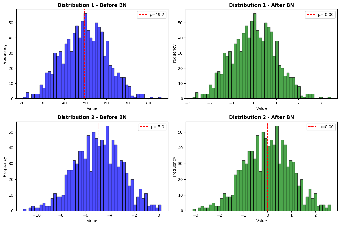
BatchNorm standardizes different distributions to similar scale
Layer Normalization#
# LayerNorm: Normalizes across features (not batch)
layer_norm = brainstate.nn.LayerNorm((10,))

print("LayerNorm:")
print(layer_norm)

# Single sample
x_single = brainstate.random.randn(10) * 5 + 10

print()
print("Before LayerNorm (single sample):")
print(f"  Values: {x_single}")
print(f"  Mean: {jnp.mean(x_single):.3f}")
print(f"  Std:  {jnp.std(x_single):.3f}")

y_single = layer_norm(x_single)

print()
print("After LayerNorm:")
print(f"  Values: {y_single}")
print(f"  Mean: {jnp.mean(y_single):.3f}")
print(f"  Std:  {jnp.std(y_single):.3f}")

print()
print("✅ LayerNorm works on single samples")
print("✅ Popular in Transformers and RNNs")
print("✅ Independent of batch size")
LayerNorm:
LayerNorm(
  in_size=(10,),
  out_size=(10,),
  feature_axes=(0,),
  reduction_axes=(-1,),
  axis_name=None,
  axis_index_groups=None,
  weight=NormalizationParamState(
    value={
      'bias': ShapedArray(float32[10]),
      'scale': ShapedArray(float32[10])
    }
  ),
  epsilon=1e-06,
  dtype=<class 'numpy.float32'>,
  use_bias=True,
  use_scale=True,
  bias_init=ZeroInit(
    unit=Unit(10.0^0)
  ),
  scale_init=Constant(
    value=1.0
  ),
  use_fast_variance=True
)

Before LayerNorm (single sample):
  Values: [ 3.0611591 13.874271  17.702465  19.20955    5.685323   5.9649186
  8.997379  13.917359   5.0701327 11.3188305]
  Mean: 10.480
  Std:  5.313

After LayerNorm:
  Values: [-1.3963605   0.6388257   1.3593478   1.6430035  -0.9024544  -0.84983045
 -0.2790769   0.64693546 -1.0182422   0.15785426]
  Mean: 0.000
  Std:  1.000

✅ LayerNorm works on single samples
✅ Popular in Transformers and RNNs
✅ Independent of batch size
Comparing Normalization Methods#
import pandas as pd

comparison = pd.DataFrame({
    'Method': ['BatchNorm', 'LayerNorm', 'GroupNorm', 'InstanceNorm'],
    'Normalizes Over': ['Batch + Spatial', 'Features', 'Groups', 'Spatial per channel'],
    'Best For': ['CNNs, large batches', 'RNNs, Transformers', 'Small batches', 'Style transfer'],
    'Batch Dependent': ['Yes', 'No', 'No', 'No'],
    'Typical Use': ['Vision', 'NLP', 'Vision (small batch)', 'GANs, Style'],
})

print("\n📊 Normalization Method Comparison:\n")
print(comparison.to_string(index=False))

print("\n\n🎯 Quick Guide:")
print("  • Large batch + CNN → BatchNorm")
print("  • Small batch + CNN → GroupNorm")
print("  • Sequences/RNN/Transformer → LayerNorm")
print("  • Single image inference → LayerNorm or GroupNorm")
📊 Normalization Method Comparison:

      Method     Normalizes Over            Best For Batch Dependent          Typical Use
   BatchNorm     Batch + Spatial CNNs, large batches             Yes               Vision
   LayerNorm            Features  RNNs, Transformers              No                  NLP
   GroupNorm              Groups       Small batches              No Vision (small batch)
InstanceNorm Spatial per channel      Style transfer              No          GANs, Style


🎯 Quick Guide:
  • Large batch + CNN → BatchNorm
  • Small batch + CNN → GroupNorm
  • Sequences/RNN/Transformer → LayerNorm
  • Single image inference → LayerNorm or GroupNorm
3. Putting It All Together#
Building a complete network with activations and normalization:
import brainunit as u


class ModernCNN(brainstate.nn.Module):
    """CNN with modern activations and normalization."""

    def __init__(self, num_classes=10):
        super().__init__()

        # Block 1: Conv + BatchNorm + GELU
        self.conv1 = brainstate.nn.Conv2d((32, 32, 3), out_channels=64, kernel_size=(3, 3), padding='SAME')
        self.bn1 = brainstate.nn.BatchNorm2d((32, 32, 64))
        self.act1 = brainstate.nn.GELU()
        self.pool1 = brainstate.nn.MaxPool2d(kernel_size=(2, 2), stride=(2, 2))

        # Block 2
        self.conv2 = brainstate.nn.Conv2d((16, 16, 64), out_channels=128, kernel_size=(3, 3), padding='SAME')
        self.bn2 = brainstate.nn.BatchNorm2d((16, 16, 128))
        self.act2 = brainstate.nn.GELU()
        self.pool2 = brainstate.nn.MaxPool2d(kernel_size=(2, 2), stride=(2, 2), in_size=self.bn2.out_size)

        # Classifier
        self.fc1 = brainstate.nn.Linear((128 * 8 * 8,), (256,))
        self.ln = brainstate.nn.LayerNorm((256,))
        self.act3 = brainstate.nn.GELU()
        self.dropout = brainstate.nn.Dropout(prob=0.5)
        self.fc2 = brainstate.nn.Linear((256,), (num_classes,))

    def update(self, x):
        # Block 1
        x = self.conv1(x)
        x = self.bn1(x)
        x = self.act1(x)
        x = self.pool1(x)

        # Block 2
        x = self.conv2(x)
        x = self.bn2(x)
        x = self.act2(x)
        x = self.pool2(x)

        # Classifier
        x = u.math.flatten(x, start_axis=1)
        x = self.fc1(x)
        x = self.ln(x)
        x = self.act3(x)
        x = self.dropout(x)
        x = self.fc2(x)

        return x

# Create and test
brainstate.random.seed(0)
model = ModernCNN(num_classes=10)

# Forward pass
x = brainstate.random.randn(4, 32, 32, 3)  # 4 images
with brainstate.environ.context(fit=True) as env:
    logits = model(x)

print("Modern CNN with GELU + BatchNorm + LayerNorm:")
print(model)
print()
print("Input:", x.shape)
print("Output:", logits.shape)
print()
print("Logits:", logits[0])
Modern CNN with GELU + BatchNorm + LayerNorm:
ModernCNN(
  conv1=Conv2d(
    in_size=(32, 32, 3),
    out_size=(32, 32, 64),
    channel_first=False,
    channels_last=True,
    in_channels=3,
    out_channels=64,
    stride=(1, 1),
    kernel_size=(3, 3),
    lhs_dilation=(1, 1),
    rhs_dilation=(1, 1),
    groups=1,
    dimension_numbers=ConvDimensionNumbers(lhs_spec=(0, 3, 1, 2), rhs_spec=(3, 2, 0, 1), out_spec=(0, 3, 1, 2)),
    padding=SAME,
    kernel_shape=(3, 3, 3, 64),
    w_mask=None,
    w_initializer=XavierNormal(
      scale=1.0,
      mode='fan_avg',
      in_axis=-2,
      out_axis=-1,
      distribution='truncated_normal',
      rng=RandomState([1846506472 1430574090]),
      unit=Unit(10.0^0)
    ),
    b_initializer=None,
    weight=ParamState(
      value={
        'weight': ShapedArray(float32[3,3,3,64])
      }
    )
  ),
  bn1=BatchNorm2d(
    in_size=(32, 32, 64),
    out_size=(32, 32, 64),
    affine=True,
    bias_initializer=Constant(
      value=0.0
    ),
    scale_initializer=Constant(
      value=1.0
    ),
    dtype=<class 'numpy.float32'>,
    track_running_stats=True,
    momentum=Array(0.99, dtype=float32),
    epsilon=Array(1.e-05, dtype=float32),
    use_fast_variance=True,
    feature_axes=(2,),
    axis_name=None,
    axis_index_groups=None,
    running_mean=BatchState(
      value=ShapedArray(float32[1,1,64])
    ),
    running_var=BatchState(
      value=ShapedArray(float32[1,1,64])
    ),
    weight=NormalizationParamState(
      value={
        'bias': ShapedArray(float32[1,1,64]),
        'scale': ShapedArray(float32[1,1,64])
      }
    )
  ),
  act1=GELU(approximate=False),
  pool1=MaxPool2d(
    init_value=-inf,
    computation=<function max at 0x000001C17F834220>,
    pool_dim=2,
    return_indices=False,
    kernel_size=(2, 2),
    stride=(2, 2),
    padding=VALID,
    channel_axis=-1
  ),
  conv2=Conv2d(
    in_size=(16, 16, 64),
    out_size=(16, 16, 128),
    channel_first=False,
    channels_last=True,
    in_channels=64,
    out_channels=128,
    stride=(1, 1),
    kernel_size=(3, 3),
    lhs_dilation=(1, 1),
    rhs_dilation=(1, 1),
    groups=1,
    dimension_numbers=ConvDimensionNumbers(lhs_spec=(0, 3, 1, 2), rhs_spec=(3, 2, 0, 1), out_spec=(0, 3, 1, 2)),
    padding=SAME,
    kernel_shape=(3, 3, 64, 128),
    w_mask=None,
    w_initializer=XavierNormal(
      scale=1.0,
      mode='fan_avg',
      in_axis=-2,
      out_axis=-1,
      distribution='truncated_normal',
      rng=RandomState([1846506472 1430574090]),
      unit=Unit(10.0^0)
    ),
    b_initializer=None,
    weight=ParamState(
      value={
        'weight': ShapedArray(float32[3,3,64,128])
      }
    )
  ),
  bn2=BatchNorm2d(
    in_size=(16, 16, 128),
    out_size=(16, 16, 128),
    affine=True,
    bias_initializer=Constant(
      value=0.0
    ),
    scale_initializer=Constant(
      value=1.0
    ),
    dtype=<class 'numpy.float32'>,
    track_running_stats=True,
    momentum=Array(0.99, dtype=float32),
    epsilon=Array(1.e-05, dtype=float32),
    use_fast_variance=True,
    feature_axes=(2,),
    axis_name=None,
    axis_index_groups=None,
    running_mean=BatchState(
      value=ShapedArray(float32[1,1,128])
    ),
    running_var=BatchState(
      value=ShapedArray(float32[1,1,128])
    ),
    weight=NormalizationParamState(
      value={
        'bias': ShapedArray(float32[1,1,128]),
        'scale': ShapedArray(float32[1,1,128])
      }
    )
  ),
  act2=GELU(approximate=False),
  pool2=MaxPool2d(
    in_size=(16, 16, 128),
    out_size=(8, 8, 128),
    init_value=-inf,
    computation=<function max at 0x000001C17F834220>,
    pool_dim=2,
    return_indices=False,
    kernel_size=(2, 2),
    stride=(2, 2),
    padding=VALID,
    channel_axis=-1
  ),
  fc1=Linear(
    in_size=(8192,),
    out_size=(256,),
    w_mask=None,
    weight=ParamState(
      value={
        'bias': ShapedArray(float32[256]),
        'weight': ShapedArray(float32[8192,256])
      }
    )
  ),
  ln=LayerNorm(
    in_size=(256,),
    out_size=(256,),
    feature_axes=(0,),
    reduction_axes=(-1,),
    axis_name=None,
    axis_index_groups=None,
    weight=NormalizationParamState(
      value={
        'bias': ShapedArray(float32[256]),
        'scale': ShapedArray(float32[256])
      }
    ),
    epsilon=1e-06,
    dtype=<class 'numpy.float32'>,
    use_bias=True,
    use_scale=True,
    bias_init=ZeroInit(
      unit=Unit(10.0^0)
    ),
    scale_init=Constant(
      value=1.0
    ),
    use_fast_variance=True
  ),
  act3=GELU(approximate=False),
  dropout=Dropout(
    prob=0.5,
    broadcast_dims=()
  ),
  fc2=Linear(
    in_size=(256,),
    out_size=(10,),
    w_mask=None,
    weight=ParamState(
      value={
        'bias': ShapedArray(float32[10]),
        'weight': ShapedArray(float32[256,10])
      }
    )
  )
)

Input: (4, 32, 32, 3)
Output: (4, 10)

Logits: [ 3.3256447  -1.429272    0.7167457   1.7075744   0.22491284 -1.362806
 -0.27098486 -0.27673492 -1.0504798  -1.4831724 ]
Summary#
In this tutorial, you learned:
✅ Activation Functions
ReLU family (ReLU, Leaky ReLU, ELU)
Modern activations (GELU, SiLU)
Classic activations (Sigmoid, Tanh)
Softmax for classification
✅ Normalization Layers
BatchNorm for large-batch training
LayerNorm for sequences and transformers
GroupNorm for small-batch scenarios
✅ Practical Guidelines
When to use each activation
When to use each normalization
How to combine them effectively
Quick Reference Card#
Task |
Activation |
Normalization |
|---|---|---|
CNN (large batch) |
ReLU/GELU |
BatchNorm |
CNN (small batch) |
ReLU/GELU |
GroupNorm |
Transformer/NLP |
GELU |
LayerNorm |
RNN/LSTM |
Tanh (gates) |
LayerNorm |
Binary output |
Sigmoid |
- |
Multi-class output |
Softmax |
- |
Best Practices#
🎯 Use ReLU/GELU as default activations
📊 Add normalization after conv/linear layers
⚡ Order: Conv/Linear → Norm → Activation
🔍 Experiment with activation functions
📝 Use appropriate normalization for your batch size
Next Steps#
Continue with:
Recurrent Networks - Handle sequential data
Training - Optimize with gradient descent
Advanced Architectures - ResNets, Transformers