
Recurrent Neural Networks#
Recurrent Neural Networks (RNNs) are designed to process sequential data by maintaining hidden states that capture temporal dependencies.
In this tutorial, you will learn:
🔄 RNN Basics - Understanding recurrence and hidden states
🧠 LSTM - Long Short-Term Memory for long-term dependencies
⚡ GRU - Gated Recurrent Unit as efficient alternative
📊 Sequence Processing - Handling variable-length sequences
💡 Practical Examples - Sentiment analysis, time series
Why RNNs?#
RNNs excel at:
📝 Natural language processing
🎵 Speech and audio
📈 Time series forecasting
🎬 Video analysis
import brainstate
import numpy as np
import jax.numpy as jnp
import matplotlib.pyplot as plt
1. RNN Basics#
An RNN processes sequences one element at a time, updating its hidden state:
h_t = tanh(W_xh @ x_t + W_hh @ h_{t-1} + b)
Simple RNN Cell#
# RNNCell: Basic recurrent unit
brainstate.random.seed(42)
rnn_cell = brainstate.nn.ValinaRNNCell(num_in=10, num_out=20)
brainstate.nn.init_all_states(rnn_cell)

print("RNNCell:")
print(rnn_cell)
print(f"Input size: {rnn_cell.in_size}")
print(f"Hidden size: {rnn_cell.out_size}")

# Process a single timestep
x_t = brainstate.random.randn(10)
hidden_before = rnn_cell.h.value
hidden_after = rnn_cell(x_t)

print(f"Input shape: {x_t.shape}")
print(f"Previous hidden shape: {hidden_before.shape}")
print(f"New hidden shape: {hidden_after.shape}")
RNNCell:
ValinaRNNCell(
  in_size=(10,),
  out_size=(20,),
  num_out=20,
  num_in=10,
  state_initializer=ZeroInit(
    unit=Unit(10.0^0)
  ),
  activation=<function relu at 0x00000135A6BE8360>,
  W=Linear(
    in_size=(30,),
    out_size=(20,),
    w_mask=None,
    weight=ParamState(
      value={
        'bias': ShapedArray(float32[20]),
        'weight': ShapedArray(float32[30,20])
      }
    )
  ),
  h=HiddenState(
    value=ShapedArray(float32[20])
  )
)
Input size: (10,)
Hidden size: (20,)
Input shape: (10,)
Previous hidden shape: (20,)
New hidden shape: (20,)
Processing Sequences#
Let’s process a complete sequence:
class SimpleRNN(brainstate.nn.Module):
    """Simple RNN for sequence processing."""

    def __init__(self, input_size, hidden_size, output_size):
        super().__init__()
        self.rnn_cell = brainstate.nn.ValinaRNNCell(num_in=input_size, num_out=hidden_size)
        self.output_layer = brainstate.nn.Linear((hidden_size,), (output_size,))
        self.hidden_size = hidden_size

    def update(self, sequence):
        # Reset recurrent state for each new sequence
        brainstate.nn.init_all_states(self)
        rnn_out = brainstate.transform.for_loop(self.rnn_cell, sequence)
        return self.output_layer(rnn_out)

# Create RNN
brainstate.random.seed(0)
rnn = SimpleRNN(input_size=5, hidden_size=10, output_size=3)

# Test sequence
sequence = brainstate.random.randn(7, 5)  # 7 timesteps, 5 features
outputs = rnn(sequence)

print(f"Input sequence shape: {sequence.shape}")
print(f"Output sequence shape: {outputs.shape}")
print(f"Outputs: {outputs}")
Input sequence shape: (7, 5)
Output sequence shape: (7, 3)
Outputs: [[ 0.02491026 -1.2344698  -0.7660187 ]
 [ 1.020083   -0.94504666  0.5592617 ]
 [ 0.5109156  -0.7276021  -0.29766443]
 [ 0.8082595   0.6000599   0.46565723]
 [ 1.1170439   0.4770828  -0.37073386]
 [ 1.4667886  -1.4823256   0.30516532]
 [ 0.7935723   0.4356203   0.21530463]]
Visualizing RNN Processing#
# Generate sine wave sequence
t = jnp.linspace(0, 4 * jnp.pi, 50)
sine_wave = jnp.sin(t)

# Prepare as sequence (add feature dimension)
sequence = sine_wave[:, None]

# Create RNN
brainstate.random.seed(42)
rnn = SimpleRNN(input_size=1, hidden_size=16, output_size=1)

# Process sequence
outputs = rnn(sequence).flatten()

# Plot
plt.figure(figsize=(12, 4))
plt.plot(t, sine_wave, linewidth=2, label='Input (Sine)', alpha=0.7)
plt.plot(t, outputs, linewidth=2, label='RNN Output', alpha=0.7)
plt.xlabel('Time')
plt.ylabel('Value')
plt.title('RNN Processing Temporal Sequence', fontweight='bold')
plt.legend()
plt.grid(alpha=0.3)
plt.show()

print("RNN learns to process temporal patterns")
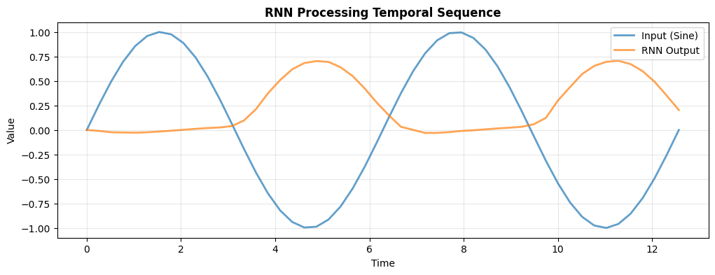
RNN learns to process temporal patterns
2. LSTM - Long Short-Term Memory#
LSTM addresses the vanishing gradient problem with gating mechanisms:
Forget gate: What to forget from cell state
Input gate: What new information to store
Output gate: What to output from cell state
LSTM Cell#
# LSTMCell: Advanced recurrent unit
brainstate.random.seed(42)
lstm_cell = brainstate.nn.LSTMCell(num_in=10, num_out=20)
brainstate.nn.init_all_states(lstm_cell)

print("LSTMCell:")
print(lstm_cell)

# LSTM has two states: hidden (h) and cell (c)
hidden_before = lstm_cell.h.value
cell_before = lstm_cell.c.value

# Process one timestep
x_t = brainstate.random.randn(10)
hidden_after = lstm_cell(x_t)
cell_after = lstm_cell.c.value

print(f"Input: {x_t.shape}")
print(f"Hidden state shape: {hidden_after.shape}")
print(f"Cell state shape: {cell_after.shape}")
print("✅ LSTM maintains both hidden and cell states")
print("✅ Cell state provides long-term memory")
LSTMCell:
LSTMCell(
  in_size=(10,),
  out_size=(20,),
  num_out=20,
  num_in=10,
  state_initializer=ZeroInit(
    unit=Unit(10.0^0)
  ),
  activation=<function tanh at 0x00000135A6BDFD80>,
  W=Linear(
    in_size=(30,),
    out_size=(80,),
    w_mask=None,
    weight=ParamState(
      value={
        'bias': ShapedArray(float32[80]),
        'weight': ShapedArray(float32[30,80])
      }
    )
  ),
  c=HiddenState(
    value=ShapedArray(float32[20])
  ),
  h=HiddenState(
    value=ShapedArray(float32[20])
  )
)
Input: (10,)
Hidden state shape: (20,)
Cell state shape: (20,)
✅ LSTM maintains both hidden and cell states
✅ Cell state provides long-term memory
LSTM Network#
class LSTMNet(brainstate.nn.Module):
    """LSTM network for sequence processing."""

    def __init__(self, input_size, hidden_size, output_size):
        super().__init__()
        self.lstm_cell = brainstate.nn.LSTMCell(num_in=input_size, num_out=hidden_size)
        self.output_layer = brainstate.nn.Linear((hidden_size,), (output_size,))
        self.hidden_size = hidden_size

    def update(self, sequence):
        brainstate.nn.init_all_states(self)
        rnn_out = brainstate.transform.for_loop(self.lstm_cell, sequence)
        return self.output_layer(rnn_out)

# Create LSTM
brainstate.random.seed(0)
lstm = LSTMNet(input_size=5, hidden_size=20, output_size=3)

# Test
sequence = brainstate.random.randn(10, 5)
outputs = lstm(sequence)

print(f"LSTM Network:")
print(lstm)
print(f"Sequence: {sequence.shape} → Output: {outputs.shape}")
LSTM Network:
LSTMNet(
  lstm_cell=LSTMCell(
    in_size=(5,),
    out_size=(20,),
    num_out=20,
    num_in=5,
    state_initializer=ZeroInit(
      unit=Unit(10.0^0)
    ),
    activation=<function tanh at 0x00000135A6BDFD80>,
    W=Linear(
      in_size=(25,),
      out_size=(80,),
      w_mask=None,
      weight=ParamState(
        value={
          'bias': ShapedArray(float32[80]),
          'weight': ShapedArray(float32[25,80])
        }
      )
    ),
    c=HiddenState(
      value=ShapedArray(float32[20])
    ),
    h=HiddenState(
      value=ShapedArray(float32[20])
    )
  ),
  output_layer=Linear(
    in_size=(20,),
    out_size=(3,),
    w_mask=None,
    weight=ParamState(
      value={
        'bias': ShapedArray(float32[3]),
        'weight': ShapedArray(float32[20,3])
      }
    )
  ),
  hidden_size=20
)
Sequence: (10, 5) → Output: (10, 3)
3. GRU - Gated Recurrent Unit#
GRU simplifies LSTM with fewer gates:
Reset gate: How much past to forget
Update gate: How much to update
GRU Cell#
# GRUCell: Efficient alternative to LSTM
brainstate.random.seed(42)
gru_cell = brainstate.nn.GRUCell(num_in=10, num_out=20)
brainstate.nn.init_all_states(gru_cell)

print("GRUCell:")
print(gru_cell)

# GRU only has hidden state (no separate cell state)
hidden_before = gru_cell.h.value
x_t = brainstate.random.randn(10)
hidden_after = gru_cell(x_t)

print(f"Input: {x_t.shape}")
print(f"Hidden state shape: {hidden_after.shape}")
print("✅ Simpler than LSTM (no cell state)")
print("✅ Faster training, fewer parameters")
print("✅ Often performs similarly to LSTM")
GRUCell:
GRUCell(
  in_size=(10,),
  out_size=(20,),
  state_initializer=ZeroInit(
    unit=Unit(10.0^0)
  ),
  num_out=20,
  num_in=10,
  activation=<function tanh at 0x00000135A6BDFD80>,
  Wrz=Linear(
    in_size=(30,),
    out_size=(40,),
    w_mask=None,
    weight=ParamState(
      value={
        'bias': ShapedArray(float32[40]),
        'weight': ShapedArray(float32[30,40])
      }
    )
  ),
  Wh=Linear(
    in_size=(30,),
    out_size=(20,),
    w_mask=None,
    weight=ParamState(
      value={
        'bias': ShapedArray(float32[20]),
        'weight': ShapedArray(float32[30,20])
      }
    )
  ),
  h=HiddenState(
    value=ShapedArray(float32[20])
  )
)
Input: (10,)
Hidden state shape: (20,)
✅ Simpler than LSTM (no cell state)
✅ Faster training, fewer parameters
✅ Often performs similarly to LSTM
Comparing RNN, LSTM, and GRU#
# Create all three types
brainstate.random.seed(0)
input_size, hidden_size = 5, 10

rnn_cell = brainstate.nn.ValinaRNNCell(num_in=input_size, num_out=hidden_size)
lstm_cell = brainstate.nn.LSTMCell(num_in=input_size, num_out=hidden_size)
gru_cell = brainstate.nn.GRUCell(num_in=input_size, num_out=hidden_size)

# Test on same sequence
sequence = brainstate.random.randn(20, input_size)

# Process with RNN
brainstate.nn.init_all_states(rnn_cell)
rnn_states = []
for x_t in sequence:
    rnn_states.append(rnn_cell(x_t))
rnn_states = jnp.stack(rnn_states)

# Process with LSTM
brainstate.nn.init_all_states(lstm_cell)
lstm_states = []
for x_t in sequence:
    lstm_states.append(lstm_cell(x_t))
lstm_states = jnp.stack(lstm_states)

# Process with GRU
brainstate.nn.init_all_states(gru_cell)
gru_states = []
for x_t in sequence:
    gru_states.append(gru_cell(x_t))
gru_states = jnp.stack(gru_states)

# Visualize hidden states
plt.figure(figsize=(15, 4))

plt.subplot(1, 3, 1)
plt.imshow(np.array(rnn_states.T), aspect='auto', cmap='viridis')
plt.colorbar()
plt.title('RNN Hidden States', fontweight='bold')
plt.xlabel('Time')
plt.ylabel('Hidden Unit')

plt.subplot(1, 3, 2)
plt.imshow(np.array(lstm_states.T), aspect='auto', cmap='viridis')
plt.colorbar()
plt.title('LSTM Hidden States', fontweight='bold')
plt.xlabel('Time')
plt.ylabel('Hidden Unit')

plt.subplot(1, 3, 3)
plt.imshow(np.array(gru_states.T), aspect='auto', cmap='viridis')
plt.colorbar()
plt.title('GRU Hidden States', fontweight='bold')
plt.xlabel('Time')
plt.ylabel('Hidden Unit')

plt.tight_layout()
plt.show()

print("Different activation patterns across time")
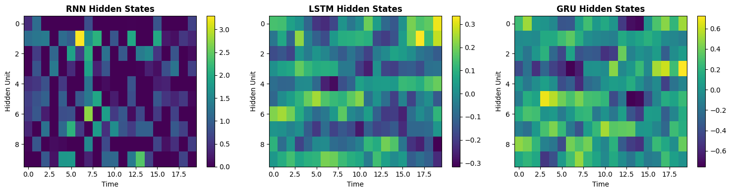
Different activation patterns across time
4. Practical Example: Sequence Classification#
Let’s build a complete sequence classifier:
class SequenceClassifier(brainstate.nn.Module):
    """Classify sequences using LSTM."""

    def __init__(self, input_size, hidden_size, num_classes):
        super().__init__()

        # LSTM layer
        self.lstm = brainstate.nn.LSTMCell(num_in=input_size, num_out=hidden_size)

        # Classifier
        self.fc = brainstate.nn.Linear((hidden_size,), (num_classes,))
        self.hidden_size = hidden_size

    def update(self, sequence):
        """Classify a sequence and return logits."""
        brainstate.nn.init_all_states(self)
        rnn_out = brainstate.transform.for_loop(self.lstm, sequence)
        return self.fc(rnn_out)

# Create classifier
brainstate.random.seed(42)
classifier = SequenceClassifier(
    input_size=8,
    hidden_size=32,
    num_classes=3
)

print("Sequence Classifier:")
print(classifier)

# Test with batch of sequences
sequences = [
    brainstate.random.randn(10, 8),  # Short sequence
    brainstate.random.randn(15, 8),  # Medium sequence
    brainstate.random.randn(20, 8),  # Long sequence
]

print("Classifying sequences of different lengths:")
for i, seq in enumerate(sequences):
    logits = classifier(seq)
    pred = jnp.argmax(logits)
    print(f"  Sequence {i + 1} (length={seq.shape[0]:2d}): logits={logits}, predicted class={pred}")
Sequence Classifier:
SequenceClassifier(
  lstm=LSTMCell(
    in_size=(8,),
    out_size=(32,),
    num_out=32,
    num_in=8,
    state_initializer=ZeroInit(
      unit=Unit(10.0^0)
    ),
    activation=<function tanh at 0x00000135A6BDFD80>,
    W=Linear(
      in_size=(40,),
      out_size=(128,),
      w_mask=None,
      weight=ParamState(
        value={
          'bias': ShapedArray(float32[128]),
          'weight': ShapedArray(float32[40,128])
        }
      )
    )
  ),
  fc=Linear(
    in_size=(32,),
    out_size=(3,),
    w_mask=None,
    weight=ParamState(
      value={
        'bias': ShapedArray(float32[3]),
        'weight': ShapedArray(float32[32,3])
      }
    )
  ),
  hidden_size=32
)
Classifying sequences of different lengths:
  Sequence 1 (length=10): logits=[[-0.01547857  0.13513905  0.00754708]
 [ 0.05315275  0.04406237 -0.03946488]
 [-0.01024249  0.01766446 -0.3073437 ]
 [-0.08865614  0.21953711 -0.22142717]
 [-0.01125905  0.23754263 -0.07070658]
 [-0.18919653  0.26399848  0.10286664]
 [-0.18127857  0.3011483   0.14584416]
 [-0.15617499  0.07344149  0.16522595]
 [-0.01809211  0.13386661  0.14542104]
 [-0.02841321  0.22150865  0.21882784]], predicted class=19
  Sequence 2 (length=15): logits=[[ 0.05904964 -0.10120873 -0.06329243]
 [ 0.17392379 -0.09240627  0.04093027]
 [ 0.18226701 -0.07839968  0.01378617]
 [ 0.17103598  0.0156443   0.07495441]
 [ 0.15527852 -0.00152822 -0.01727968]
 [-0.03237936 -0.12036745 -0.09828403]
 [-0.06232247 -0.05956251  0.05448275]
 [-0.08484429  0.02086652  0.02134096]
 [-0.04571725  0.0271459  -0.03105914]
 [ 0.03056999  0.03487205 -0.06918844]
 [ 0.10113777  0.07460307 -0.22886036]
 [-0.03290576  0.01573478 -0.23962773]
 [ 0.01381631  0.01904286 -0.24691448]
 [ 0.00996852  0.1708695  -0.21775015]
 [-0.07599682  0.10057165 -0.13780987]], predicted class=6
  Sequence 3 (length=20): logits=[[-0.03186802 -0.02496959 -0.09452604]
 [ 0.06142969 -0.00672111 -0.16893423]
 [ 0.08336904  0.19765691 -0.03138714]
 [ 0.20414184  0.17294948 -0.01703165]
 [ 0.12318151  0.10354187 -0.13263148]
 [-0.06375938 -0.08475278 -0.17380428]
 [-0.01210234 -0.14016798 -0.17115496]
 [ 0.04803856 -0.05086609 -0.28233108]
 [ 0.07683823 -0.08949272 -0.2292438 ]
 [ 0.06163431 -0.19596225 -0.25488782]
 [-0.03754998 -0.4479535  -0.2219074 ]
 [ 0.01833916 -0.40765774 -0.1654255 ]
 [-0.01680591 -0.23481718  0.03301343]
 [ 0.00481436 -0.1791741  -0.0043909 ]
 [-0.02281204 -0.07078494  0.00409675]
 [-0.10403152 -0.07854924 -0.0093255 ]
 [-0.04130641 -0.01892788  0.07624298]
 [-0.09435351  0.02813931  0.19073027]
 [ 0.02372409  0.02199761  0.17838839]
 [-0.00277933  0.20082155  0.1791797 ]], predicted class=9
5. Time Series Prediction#
# Generate synthetic time series
def generate_time_series(n_steps=100):
    t = jnp.linspace(0, 10, n_steps)
    # Combination of sine waves
    series = jnp.sin(t) + 0.5 * jnp.sin(3 * t) + 0.1 * brainstate.random.randn(n_steps)
    return series

# Create sequences for prediction
def create_sequences(data, seq_length=10):
    X, y = [], []
    for i in range(len(data) - seq_length):
        X.append(data[i:i + seq_length])
        y.append(data[i + seq_length])
    return jnp.array(X), jnp.array(y)

# Generate data
brainstate.random.seed(0)
time_series = generate_time_series(200)
X, y = create_sequences(time_series, seq_length=15)

# Add feature dimension
X = X[:, :, None]

print(f"Time series data: {time_series.shape}")
print(f"Sequences (X): {X.shape}")
print(f"Targets (y): {y.shape}")

# Create predictor
class TimeSeriesPredictor(brainstate.nn.Module):
    def __init__(self, hidden_size=32):
        super().__init__()
        self.gru = brainstate.nn.GRUCell(num_in=1, num_out=hidden_size)
        self.fc = brainstate.nn.Linear((hidden_size,), (1,))
        self.hidden_size = hidden_size

    def update(self, sequence):
        brainstate.nn.init_all_states(self)
        brainstate.transform.for_loop(self.gru, sequence)
        prediction = self.fc(self.gru.h.value)
        return prediction.squeeze()

# Create and test predictor
brainstate.random.seed(42)
predictor = TimeSeriesPredictor(hidden_size=64)

# Make predictions on test data
predictions = []
for i in range(min(50, len(X))):
    pred = predictor(X[i])
    predictions.append(pred)

predictions = jnp.array(predictions)
targets = y[:len(predictions)]

# Plot
plt.figure(figsize=(12, 5))
plt.plot(targets, label='True Values', linewidth=2, alpha=0.7)
plt.plot(predictions, label='Predictions (Untrained)', linewidth=2, alpha=0.7)
plt.xlabel('Time Step')
plt.ylabel('Value')
plt.title('Time Series Prediction with GRU', fontweight='bold')
plt.legend()
plt.grid(alpha=0.3)
plt.show()

mse = jnp.mean((predictions - targets) ** 2)
print(f"MSE (untrained): {mse:.4f}")
print("💡 With training, GRU can learn to predict future values")
Time series data: (200,)
Sequences (X): (185, 15, 1)
Targets (y): (185,)
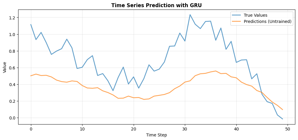
MSE (untrained): 0.1451
💡 With training, GRU can learn to predict future values
Summary#
In this tutorial, you learned:
✅ RNN Basics
Recurrence and hidden states
Processing sequences step-by-step
Building simple RNN networks
✅ LSTM
Gating mechanisms (forget, input, output)
Cell state for long-term memory
Handling long-term dependencies
✅ GRU
Simplified gating (reset, update)
Fewer parameters than LSTM
Efficient alternative
✅ Practical Applications
Sequence classification
Time series prediction
Variable-length sequences
Quick Comparison#
Model |
States |
Gates |
Best For |
|---|---|---|---|
RNN |
1 (h) |
0 |
Short sequences, simple patterns |
LSTM |
2 (h, c) |
3 |
Long sequences, complex dependencies |
GRU |
1 (h) |
2 |
Balance of complexity and performance |
When to Use Each#
🎯 Start with GRU - Good default choice
📚 Use LSTM - When you need maximum capacity for long-term memory
⚡ Use RNN - For simple patterns or as baseline
Best Practices#
🔄 Initialize hidden states to zero
📊 Normalize input sequences
🎯 Use gradient clipping to prevent exploding gradients
💾 Save hidden states for inference on long sequences
🔍 Try bidirectional RNNs for offline sequence processing
Next Steps#
Continue with:
Dynamics Systems - Brain-inspired temporal models
Attention Mechanisms - Beyond RNNs (Transformers)
Training - Optimize RNNs effectively