Delay Protocol

Introduction

Delays are fundamental in neural systems, arising from:

• Axonal conduction delays: Signal propagation along axons takes time

• Synaptic delays: Chemical transmission across synapses introduces latency

• Network delays: Multi-step information processing creates temporal lags

BrainState provides three powerful APIs for handling delays:

1. brainstate.nn.Delay: General-purpose delay buffer for any data

2. brainstate.nn.DelayAccess: Named accessor for specific delay entries

3. brainstate.nn.StateWithDelay: Automatic delay tracking for module states

Learning Objectives

By the end of this tutorial, you will:

• ✅ Understand the two delay buffer methods: rotation vs concatenation

• ✅ Use Delay to create flexible delay buffers with multiple delay taps

• ✅ Access delayed values using DelayAccess and named entries

• ✅ Leverage StateWithDelay for automatic state history tracking

• ✅ Implement realistic neural models with synaptic and axonal delays

• ✅ Choose between step-based and time-based delay retrieval

• ✅ Use linear vs round interpolation for continuous-time delays

---

Setup

import brainstate
import brainunit as u
import jax.numpy as jnp
import matplotlib.pyplot as plt

brainstate.environ.set(dt=0.1 * u.ms)  # 0.1 ms time step

---

Part 1: Understanding brainstate.nn.Delay

1.1 What is a Delay Buffer?

A delay buffer stores a rolling history of values over time. Think of it as a time window looking into the past:

Time:  t-3    t-2    t-1    t (now)
       │      │      │      │
Data:  [10] → [20] → [30] → [40]
       ↑      ↑      ↑      ↑
     delay=3 delay=2 delay=1 delay=0

The Delay class maintains this history efficiently using two methods:

1. Rotation method (default): Uses a ring buffer with modulo indexing

2. Concatenation method: Shifts data by concatenating new values

1.2 Creating a Basic Delay

Let’s create a simple delay buffer for a scalar signal:

# Create a delay buffer for a scalar value
# We need to specify the shape/dtype of data we'll store
target_data = jnp.array([0.0])  # Example: scalar in array form

# Create delay with 5ms maximum delay
delay_buffer = brainstate.nn.Delay(
    target_info=target_data,  # Shape/dtype template
    time=5.0 * u.ms,          # Maximum delay time
    init=0.0,                 # Initial history value
    delay_method='rotation'   # Use ring buffer (default)
)

# Initialize the state
delay_buffer.init_state()

print(f"Maximum delay time: {delay_buffer.max_time}")
print(f"Maximum delay length (steps): {delay_buffer.max_length}")
print(f"History buffer shape: {delay_buffer.history.value.shape}")

Maximum delay time: 5.0 * msecond
Maximum delay length (steps): 51
History buffer shape: (51, 1)

1.3 Registering Delay Entries

You can register multiple named entries for different delay times:

# Create delay buffer with multiple taps
delay_buffer = brainstate.nn.Delay(
    target_info=jnp.array([0.0]),
    time=10.0 * u.ms,  # Support delays up to 10ms
    init=0.0
)

# Register different delay times with names
delay_buffer.register_entry('immediate', 0.0 * u.ms)   # No delay
delay_buffer.register_entry('short', 2.0 * u.ms)       # 2ms delay
delay_buffer.register_entry('medium', 5.0 * u.ms)      # 5ms delay
delay_buffer.register_entry('long', 10.0 * u.ms)       # 10ms delay

delay_buffer.init_state()

print("Registered delay entries:")
for name, delay_info in delay_buffer._registered_entries.items():
    print(f"  {name}: {delay_info} steps")

Registered delay entries:
  immediate: (Array(0, dtype=int32),) steps
  short: (Array(20, dtype=int32),) steps
  medium: (Array(50, dtype=int32),) steps
  long: (Array(100, dtype=int32),) steps

1.4 Updating and Accessing Delayed Values

Now let’s simulate a signal and access its delayed versions:

# Simulation parameters
duration = 50.0 * u.ms
dt = brainstate.environ.get_dt()
num_steps = int(duration / dt)

# Storage for visualization
times = []
current_values = []
delayed_short = []
delayed_medium = []
delayed_long = []

# Simulate a sinusoidal signal
for i in range(num_steps):
    t = i * dt
    brainstate.environ.set(i=i, t=t)
    
    # Current signal: sin(2π * 50Hz * t)
    current = jnp.sin(2 * jnp.pi * 50.0 * (t / u.second)) 
    current_array = jnp.array([current])
    
    # Update delay buffer with current value
    delay_buffer.update(current_array)
    
    # Retrieve delayed values
    val_immediate = delay_buffer.at('immediate')[0]
    val_short = delay_buffer.at('short')[0]
    val_medium = delay_buffer.at('medium')[0]
    val_long = delay_buffer.at('long')[0]
    
    # Store for plotting
    times.append(float(t / u.ms))
    current_values.append(float(val_immediate))
    delayed_short.append(float(val_short))
    delayed_medium.append(float(val_medium))
    delayed_long.append(float(val_long))

# Visualize
plt.figure(figsize=(12, 6))
plt.plot(times, current_values, label='Current (0ms delay)', linewidth=2)
plt.plot(times, delayed_short, label='Short (2ms delay)', alpha=0.7)
plt.plot(times, delayed_medium, label='Medium (5ms delay)', alpha=0.7)
plt.plot(times, delayed_long, label='Long (10ms delay)', alpha=0.7)
plt.xlabel('Time (ms)')
plt.ylabel('Signal Value')
plt.title('Delay Buffer: Multiple Delay Taps on 50Hz Sinusoid')
plt.legend()
plt.grid(True, alpha=0.3)
plt.tight_layout()
plt.show()

print("✅ Delay buffer successfully stores and retrieves delayed values")

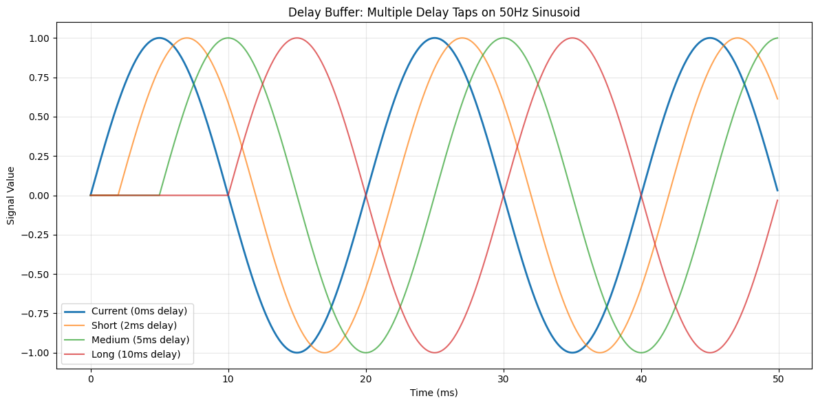
✅ Delay buffer successfully stores and retrieves delayed values

1.5 Rotation vs Concatenation Methods

Rotation method (ring buffer):

• More memory efficient

• Uses modulo indexing: index = (current_step - delay_step) % max_length

• Default and recommended for most cases

Concatenation method:

• Shifts entire buffer on each update

• Easier to understand conceptually

• Can be slower for large buffers

Let’s compare both:

# Create two delay buffers with different methods
delay_rotation = brainstate.nn.Delay(
    target_info=jnp.array([0.0]),
    time=5.0 * u.ms,
    delay_method='rotation'
)
delay_rotation.register_entry('test', 3.0 * u.ms)
delay_rotation.init_state()

delay_concat = brainstate.nn.Delay(
    target_info=jnp.array([0.0]),
    time=5.0 * u.ms,
    delay_method='concat'
)
delay_concat.register_entry('test', 3.0 * u.ms)
delay_concat.init_state()

# Simulate 10 steps
print("Comparing rotation vs concatenation methods:\n")
for i in range(10):
    brainstate.environ.set(i=i)
    
    # Update both with same value
    value = jnp.array([float(i)])
    delay_rotation.update(value)
    delay_concat.update(value)
    
    # Retrieve delayed values
    val_rotation = delay_rotation.at('test')[0]
    val_concat = delay_concat.at('test')[0]
    
    print(f"Step {i}: Rotation={val_rotation:.1f}, Concat={val_concat:.1f}, Match={jnp.allclose(val_rotation, val_concat)}")

print("\n✅ Both methods produce identical results")

Comparing rotation vs concatenation methods:

Step 0: Rotation=0.0, Concat=0.0, Match=True
Step 1: Rotation=0.0, Concat=0.0, Match=True
Step 2: Rotation=0.0, Concat=0.0, Match=True
Step 3: Rotation=0.0, Concat=0.0, Match=True
Step 4: Rotation=0.0, Concat=0.0, Match=True
Step 5: Rotation=0.0, Concat=0.0, Match=True
Step 6: Rotation=0.0, Concat=0.0, Match=True
Step 7: Rotation=0.0, Concat=0.0, Match=True
Step 8: Rotation=0.0, Concat=0.0, Match=True
Step 9: Rotation=0.0, Concat=0.0, Match=True

✅ Both methods produce identical results

---

Part 2: Time-based vs Step-based Retrieval

2.1 Step-based Retrieval

When you know the exact delay in integer time steps, use retrieve_at_step():

delay_buffer = brainstate.nn.Delay(
    target_info=jnp.array([0.0]),
    time=10.0 * u.ms,
)
delay_buffer.init_state()

# Populate buffer
for i in range(20):
    brainstate.environ.set(i=i)
    delay_buffer.update(jnp.array([float(i * 10)]))

# Retrieve by step (integer delay)
brainstate.environ.set(i=19)  # At step 19
current = delay_buffer.retrieve_at_step(0)      # 0 steps back
delayed_5 = delay_buffer.retrieve_at_step(5)    # 5 steps back
delayed_10 = delay_buffer.retrieve_at_step(10)  # 10 steps back

print("Step-based retrieval at step 19:")
print(f"  0 steps back (current):  {current[0]:.1f} (expected: {19*10})")
print(f"  5 steps back:            {delayed_5[0]:.1f} (expected: {(19-5)*10})")
print(f"  10 steps back:           {delayed_10[0]:.1f} (expected: {(19-10)*10})")

Step-based retrieval at step 19:
  0 steps back (current):  190.0 (expected: 190)
  5 steps back:            140.0 (expected: 140)
  10 steps back:           90.0 (expected: 90)

2.2 Time-based Retrieval

When delays are specified in continuous time, use retrieve_at_time(). This supports interpolation:

# Create delay with linear interpolation
delay_linear = brainstate.nn.Delay(
    target_info=jnp.array([0.0]),
    time=5.0 * u.ms,
    interp_method='linear_interp'  # Linear interpolation
)
delay_linear.init_state()

# Create delay with round interpolation
delay_round = brainstate.nn.Delay(
    target_info=jnp.array([0.0]),
    time=5.0 * u.ms,
    interp_method='round'  # Round to nearest step
)
delay_round.init_state()

# Populate both buffers
for i in range(100):
    t = i * brainstate.environ.get_dt()
    brainstate.environ.set(i=i, t=t)
    value = jnp.array([float(i)])
    delay_linear.update(value)
    delay_round.update(value)

# Retrieve at non-integer delay times
t_current = 99 * brainstate.environ.get_dt()
brainstate.environ.set(i=99, t=t_current)

delay_time = 2.5 * u.ms  # 2.5ms = 25 steps (non-integer at 0.1ms resolution)
target_time = t_current - delay_time

val_linear = delay_linear.retrieve_at_time(target_time)[0]
val_round = delay_round.retrieve_at_time(target_time)[0]

print(f"Time-based retrieval at t={float(t_current / u.ms):.1f}ms, delay={float(delay_time / u.ms)}ms:")
print(f"  Linear interpolation: {val_linear:.2f} (between steps 74 and 75)")
print(f"  Round interpolation:  {val_round:.2f} (rounds to nearest step)")
print(f"  Expected exact value: {99 - 25} (25 steps back from step 99)")

Time-based retrieval at t=9.9ms, delay=2.5ms:
  Linear interpolation: 74.00 (between steps 74 and 75)
  Round interpolation:  74.00 (rounds to nearest step)
  Expected exact value: 74 (25 steps back from step 99)

2.3 Interpolation Comparison

Let’s visualize the difference between linear and round interpolation:

# Create delays with different interpolation
delay_linear = brainstate.nn.Delay(jnp.array([0.0]), time=10.0 * u.ms, interp_method='linear_interp')
delay_round = brainstate.nn.Delay(jnp.array([0.0]), time=10.0 * u.ms, interp_method='round')
delay_linear.init_state()
delay_round.init_state()

# Populate with ramp signal
for i in range(200):
    t = i * brainstate.environ.get_dt()
    brainstate.environ.set(i=i, t=t)
    value = jnp.array([float(i)])
    delay_linear.update(value)
    delay_round.update(value)

# Test various delay times (non-integer steps)
t_now = 199 * brainstate.environ.get_dt()
brainstate.environ.set(i=199, t=t_now)

delay_times_ms = jnp.linspace(0.0, 10.0, 101)  # 0 to 10ms
linear_vals = []
round_vals = []

for delay_ms in delay_times_ms:
    delay_time = delay_ms * u.ms
    target_time = t_now - delay_time
    
    val_linear = delay_linear.retrieve_at_time(target_time)[0]
    val_round = delay_round.retrieve_at_time(target_time)[0]
    
    linear_vals.append(float(val_linear))
    round_vals.append(float(val_round))

plt.figure(figsize=(12, 5))
plt.plot(delay_times_ms, linear_vals, label='Linear Interpolation', linewidth=2)
plt.plot(delay_times_ms, round_vals, label='Round Interpolation', linewidth=2, alpha=0.7, linestyle='--')
plt.xlabel('Delay Time (ms)')
plt.ylabel('Retrieved Value')
plt.title('Linear vs Round Interpolation in Time-based Delay Retrieval')
plt.legend()
plt.grid(True, alpha=0.3)
plt.tight_layout()
plt.show()

print("✅ Linear interpolation provides smooth continuous values")
print("✅ Round interpolation snaps to nearest discrete time step")

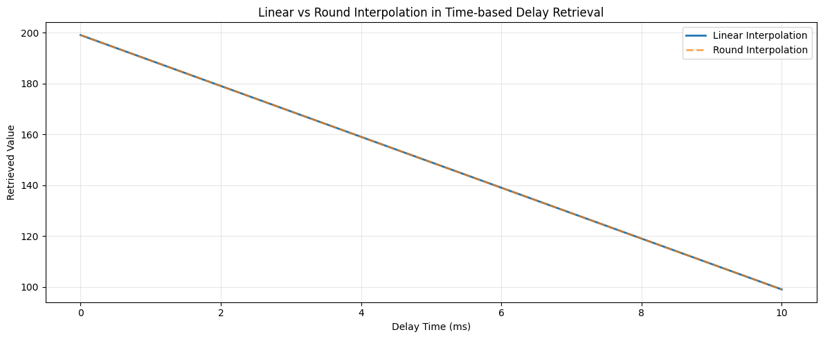
✅ Linear interpolation provides smooth continuous values
✅ Round interpolation snaps to nearest discrete time step

---

Part 3: brainstate.nn.DelayAccess

3.1 What is DelayAccess?

DelayAccess creates a reusable accessor for a specific delay entry. It’s useful when:

• You need to pass delay accessors to other modules

• You want to encapsulate delay configuration

• Building modular neural network components

3.2 Creating and Using DelayAccess

# Create a delay buffer
delay_buffer = brainstate.nn.Delay(
    target_info=jnp.array([0.0, 0.0, 0.0]),  # 3D vector
    time=10.0 * u.ms,
)
delay_buffer.init_state()

# Create DelayAccess objects for different delays
# Method 1: Using .access() method
accessor_2ms = delay_buffer.access('entry_2ms', 2.0 * u.ms)
accessor_5ms = delay_buffer.access('entry_5ms', 5.0 * u.ms)

# Simulate signal
for i in range(200):
    brainstate.environ.set(i=i)
    
    # Update with [i, i*2, i*3]
    value = jnp.array([float(i), float(i*2), float(i*3)])
    delay_buffer.update(value)

# Access delayed values through DelayAccess objects
delayed_2ms = accessor_2ms.update()  # Call update() to retrieve
delayed_5ms = accessor_5ms.update()

print("DelayAccess retrieval at step 199:")
print(f"  2ms delay (20 steps): {delayed_2ms}")
print(f"  5ms delay (50 steps): {delayed_5ms}")
print(f"  Expected 2ms: [{199-20}, {(199-20)*2}, {(199-20)*3}]")
print(f"  Expected 5ms: [{199-50}, {(199-50)*2}, {(199-50)*3}]")

DelayAccess retrieval at step 199:
  2ms delay (20 steps): [179. 358. 537.]
  5ms delay (50 steps): [149. 298. 447.]
  Expected 2ms: [179, 358, 537]
  Expected 5ms: [149, 298, 447]

3.3 Using DelayAccess in Modules

DelayAccess is particularly useful when building modular components:

class DelayedConnection(brainstate.nn.Module):
    """A module that applies delayed weighted connection."""
    
    def __init__(self, size, weight, delay_time):
        super().__init__()
        self.weight = weight
        
        # Create delay buffer and accessor
        self.delay_buffer = brainstate.nn.Delay(
            target_info=jnp.zeros(size),
            time=delay_time * 2,  # Buffer size
        )
        self.delay_access = self.delay_buffer.access('conn', delay_time)
    
    def update(self, current_input):
        # Store current input
        self.delay_buffer.update(current_input)
        
        # Get delayed input
        delayed_input = self.delay_access.update()
        
        # Apply weight to delayed input
        return self.weight * delayed_input

# Create delayed connection
conn = DelayedConnection(size=5, weight=0.5, delay_time=3.0 * u.ms)
conn.delay_buffer.init_state()

# Simulate
print("Testing DelayedConnection module:\n")
for i in range(50):
    brainstate.environ.set(i=i)
    
    # Input: [i, i, i, i, i]
    input_signal = jnp.ones(5) * i
    output = conn.update(input_signal)
    
    if i % 10 == 0:
        print(f"Step {i:2d}: Input={float(input_signal[0]):5.1f}, Output={float(output[0]):5.1f}")

print("\n✅ DelayAccess enables modular delay handling in custom modules")

Testing DelayedConnection module:

Step  0: Input=  0.0, Output=  0.0
Step 10: Input= 10.0, Output=  0.0
Step 20: Input= 20.0, Output=  0.0
Step 30: Input= 30.0, Output=  0.0
Step 40: Input= 40.0, Output=  5.0

✅ DelayAccess enables modular delay handling in custom modules

---

Part 4: brainstate.nn.StateWithDelay

4.1 What is StateWithDelay?

StateWithDelay is a specialized delay that automatically tracks a State variable in a module:

• Automatically bound to a module’s state (e.g., membrane potential V)

• Updates history buffer after each simulation step

• Commonly created via prefetch_delay() helper

• Ideal for delayed feedback and recurrent connections

4.2 Using StateWithDelay via prefetch_delay()

The easiest way to use StateWithDelay is through the Dynamics prefetch_delay() method:

class LIFWithDelayedFeedback(brainstate.nn.Dynamics):
    """LIF neuron with delayed self-feedback."""
    
    def __init__(self, size, feedback_delay=5.0 * u.ms, feedback_strength=0.3):
        super().__init__(in_size=size)
        
        # Neuron parameters
        self.tau = 10.0 * u.ms
        self.V_rest = -65.0 * u.mV
        self.V_th = -50.0 * u.mV
        self.V_reset = -65.0 * u.mV
        self.R = 1.0 * u.ohm
        self.feedback_strength = feedback_strength
        
        # States
        self.V = brainstate.State(jnp.ones(size) * self.V_rest)
        self.spike = brainstate.State(jnp.zeros(size, dtype=bool))
        
        # Create StateWithDelay for V using prefetch_delay()
        # This automatically creates a StateWithDelay and registers it
        self.V_delayed = self.prefetch_delay('V', feedback_delay)
    
    def update(self, I):
        # Get delayed voltage for feedback
        V_delayed = self.V_delayed()  # Call to retrieve delayed value
        
        # Add delayed feedback to input current
        feedback_current = (V_delayed - self.V_rest) * self.feedback_strength / self.R
        I_total = I + feedback_current
        
        # Update voltage (exponential Euler)
        dt = brainstate.environ.get_dt()
        alpha = jnp.exp(-dt / self.tau)
        V_inf = self.V_rest + I_total * self.R
        self.V.value = self.V.value * alpha + V_inf * (1 - alpha)
        
        # Spike detection and reset
        self.spike.value = self.V.value >= self.V_th
        self.V.value = u.math.where(self.spike.value, self.V_reset, self.V.value)
        
        return self.spike.value

# Create neuron with delayed feedback
neuron = LIFWithDelayedFeedback(size=1, feedback_delay=3.0 * u.ms, feedback_strength=0.4)
brainstate.nn.init_all_states(neuron)

# Simulate
duration = 100.0 * u.ms
num_steps = int(duration / brainstate.environ.get_dt())

times = []
voltages = []
spikes = []

for i in range(num_steps):
    t = i * brainstate.environ.get_dt()
    brainstate.environ.set(i=i, t=t)
    
    # Constant input current
    I_input = 1.5 * u.nA * jnp.ones(1)
    
    spike_output = neuron.update(I_input)
    
    times.append(float(t / u.ms))
    voltages.append(float(neuron.V.value[0] / u.mV))
    spikes.append(float(spike_output[0]))

# Visualize
fig, (ax1, ax2) = plt.subplots(2, 1, figsize=(12, 6), sharex=True)

# Voltage trace
ax1.plot(times, voltages, linewidth=1.5)
ax1.axhline(y=-50.0, color='r', linestyle='--', alpha=0.5, label='Threshold')
ax1.set_ylabel('Membrane Potential (mV)')
ax1.set_title('LIF Neuron with Delayed Self-Feedback (3ms delay)')
ax1.legend()
ax1.grid(True, alpha=0.3)

# Spike raster
spike_times = [times[i] for i in range(len(spikes)) if spikes[i] > 0.5]
ax2.eventplot([spike_times], lineoffsets=0.5, linelengths=0.8, colors='red')
ax2.set_ylabel('Spikes')
ax2.set_xlabel('Time (ms)')
ax2.set_ylim([0, 1])
ax2.set_yticks([])
ax2.grid(True, alpha=0.3)

plt.tight_layout()
plt.show()

print("✅ StateWithDelay automatically tracks module states for delayed feedback")

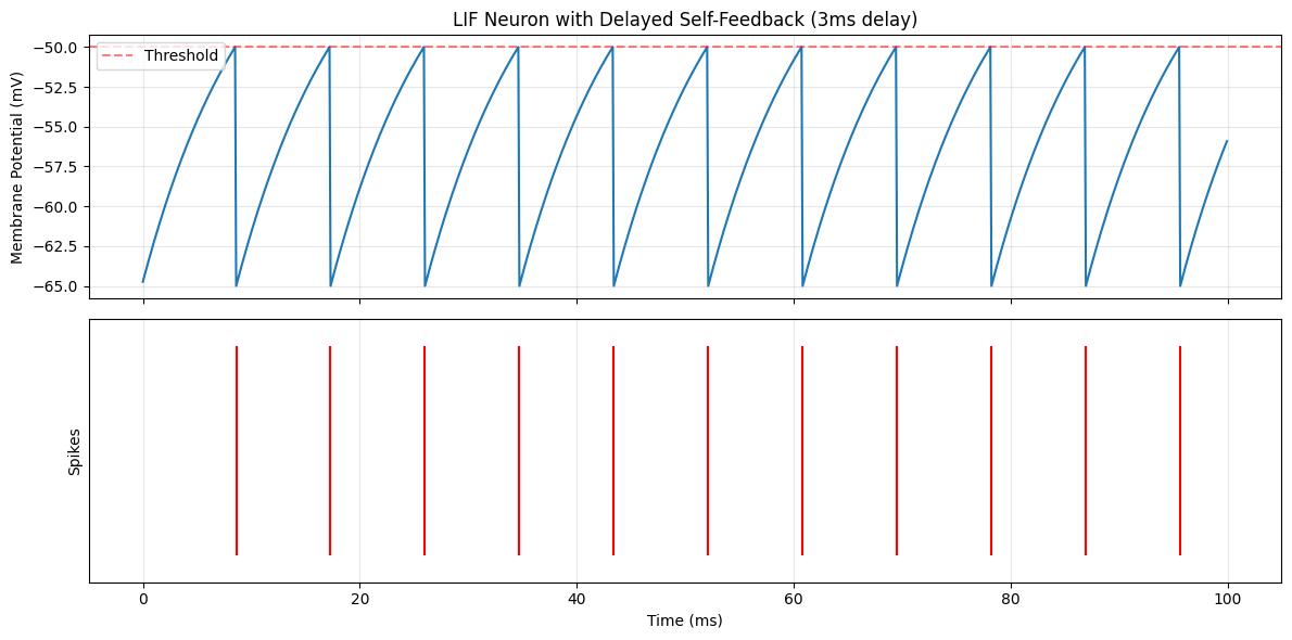
✅ StateWithDelay automatically tracks module states for delayed feedback

4.3 Direct StateWithDelay Creation

You can also create StateWithDelay explicitly (advanced usage):

class SimpleNeuron(brainstate.nn.Dynamics):
    """Simple neuron for demonstration."""
    
    def __init__(self, size):
        super().__init__(in_size=size)
        self.V = brainstate.State(jnp.zeros(size))
    
    def update(self, x):
        self.V.value = self.V.value * 0.9 + x
        return self.V.value

# Create neuron
neuron = SimpleNeuron(size=3)
neuron.init_state()

# Manually create StateWithDelay for neuron.V
state_delay = brainstate.nn.StateWithDelay(
    target=neuron,          # The module owning the state
    item='V',               # Name of the state attribute
    delay_method='rotation'
)

# Register a delay time
state_delay.register_entry('V_5ms', 5.0 * u.ms)

# Initialize
state_delay.init_state()

# Simulate
print("Manual StateWithDelay creation:\n")
for i in range(100):
    brainstate.environ.set(i=i)
    
    # Update neuron
    neuron.update(jnp.array([1.0, 2.0, 3.0]) * (i / 10.0))
    
    # Update delay buffer (must be done manually in this case)
    state_delay.update()
    
    if i % 20 == 0:
        current_V = neuron.V.value
        delayed_V = state_delay.at('V_5ms')
        print(f"Step {i:3d}: Current V={current_V}, Delayed V={delayed_V}")

print("\n✅ StateWithDelay can be created explicitly for fine-grained control")

Manual StateWithDelay creation:

Step   0: Current V=[0. 0. 0.], Delayed V=[0. 0. 0.]
Step  20: Current V=[12.094189 24.188377 36.282566], Delayed V=[0. 0. 0.]
Step  40: Current V=[31.133022 62.266045 93.39906 ], Delayed V=[0. 0. 0.]
Step  60: Current V=[ 51.016167 102.03233  153.0485  ], Delayed V=[ 4.1381054  8.276211  12.414316 ]
Step  80: Current V=[ 71.00195 142.0039  213.00584], Delayed V=[21.381517 42.763035 64.14455 ]

✅ StateWithDelay can be created explicitly for fine-grained control

---

Part 5: Practical Example - Synaptic Transmission with Delays

Let’s build a realistic synapse model with axonal and dendritic delays:

5.1 Delayed Synaptic Connection

class SimpleLIF(brainstate.nn.Dynamics):
    """Simple LIF neuron."""
    
    def __init__(self, size, tau=10.0 * u.ms, V_rest=-65.0 * u.mV,
                 V_th=-50.0 * u.mV, V_reset=-65.0 * u.mV, R=1.0 * u.ohm):
        super().__init__(in_size=size)
        
        self.tau = tau
        self.V_rest = V_rest
        self.V_th = V_th
        self.V_reset = V_reset
        self.R = R
        
        self.V = brainstate.State(jnp.ones(size) * V_rest)
        self.spike = brainstate.State(jnp.zeros(size, dtype=bool))
    
    def update(self, I):
        dt = brainstate.environ.get_dt()
        alpha = jnp.exp(-dt / self.tau)
        
        V_inf = self.V_rest + I * self.R
        self.V.value = self.V.value * alpha + V_inf * (1 - alpha)
        
        self.spike.value = self.V.value >= self.V_th
        self.V.value = u.math.where(self.spike.value, self.V_reset, self.V.value)
        
        return self.spike.value


class DelayedSynapse(brainstate.nn.Dynamics):
    """Synapse with conduction delay."""
    
    def __init__(self, pre_size, post_size, weight_matrix, 
                 axonal_delay=2.0 * u.ms, tau_syn=5.0 * u.ms):
        super().__init__(in_size=pre_size)
        
        self.weight = weight_matrix
        self.tau_syn = tau_syn
        
        # Synaptic current state
        self.I_syn = brainstate.State(jnp.zeros(post_size) * u.mA)
        
        # Create delay buffer for presynaptic spikes
        self.spike_delay = brainstate.nn.Delay(
            target_info=jnp.zeros(pre_size, dtype=bool),
            time=axonal_delay * 2,
            init=False
        )
        self.spike_delay.register_entry('axonal', axonal_delay)
    
    def update(self, pre_spike):
        # Store presynaptic spikes
        self.spike_delay.update(pre_spike)
        
        # Retrieve delayed spikes
        delayed_spike = self.spike_delay.at('axonal')
        
        # Synaptic current injection
        I_input = self.weight @ delayed_spike.astype(jnp.float32)
        
        # Synaptic current decay
        dt = brainstate.environ.get_dt()
        alpha = jnp.exp(-dt / self.tau_syn)
        self.I_syn.value = self.I_syn.value * alpha + I_input
        
        return self.I_syn.value


# Create network: pre -> synapse -> post
pre_neuron = SimpleLIF(size=1)
post_neuron = SimpleLIF(size=1)

# Synaptic weight
weight = jnp.array([[2.0]]) * u.mA  # Strong connection

synapse = DelayedSynapse(
    pre_size=1, 
    post_size=1, 
    weight_matrix=weight,
    axonal_delay=5.0 * u.ms,  # 5ms axonal delay
    tau_syn=3.0 * u.ms
)

# Initialize
pre_neuron.init_state()
post_neuron.init_state()
synapse.spike_delay.init_state()

# Simulate
duration = 100.0 * u.ms
num_steps = int(duration / brainstate.environ.get_dt())

times = []
pre_voltages = []
post_voltages = []
syn_currents = []
pre_spikes = []
post_spikes = []

for i in range(num_steps):
    t = i * brainstate.environ.get_dt()
    brainstate.environ.set(i=i, t=t)
    
    # Strong input to presynaptic neuron
    I_pre = 20. * u.mA * jnp.ones(1)
    
    # Update presynaptic neuron
    pre_spike = pre_neuron.update(I_pre)
    
    # Update synapse with delayed transmission
    I_syn = synapse.update(pre_spike)
    
    # Update postsynaptic neuron
    post_spike = post_neuron.update(I_syn)
    
    # Record
    times.append(float(t / u.ms))
    pre_voltages.append(float(pre_neuron.V.value[0] / u.mV))
    post_voltages.append(float(post_neuron.V.value[0] / u.mV))
    syn_currents.append(float(I_syn[0] / u.nA))
    pre_spikes.append(float(pre_spike[0]))
    post_spikes.append(float(post_spike[0]))

# Visualize
fig, axes = plt.subplots(4, 1, figsize=(14, 10), sharex=True)

# Presynaptic voltage
axes[0].plot(times, pre_voltages, 'b', linewidth=1.5)
axes[0].axhline(y=-50.0, color='r', linestyle='--', alpha=0.5)
axes[0].set_ylabel('Pre V (mV)')
axes[0].set_title('Synaptic Transmission with 5ms Axonal Delay')
axes[0].grid(True, alpha=0.3)

# Presynaptic spikes
pre_spike_times = [times[i] for i in range(len(pre_spikes)) if pre_spikes[i] > 0.5]
axes[1].eventplot([pre_spike_times], lineoffsets=0.5, linelengths=0.8, colors='blue')
axes[1].set_ylabel('Pre Spikes')
axes[1].set_ylim([0, 1])
axes[1].set_yticks([])
axes[1].grid(True, alpha=0.3)

# Synaptic current
axes[2].plot(times, syn_currents, 'g', linewidth=1.5)
axes[2].set_ylabel('Syn Current (nA)')
axes[2].grid(True, alpha=0.3)

# Postsynaptic voltage
axes[3].plot(times, post_voltages, 'r', linewidth=1.5)
axes[3].axhline(y=-50.0, color='r', linestyle='--', alpha=0.5)
axes[3].set_ylabel('Post V (mV)')
axes[3].set_xlabel('Time (ms)')
axes[3].grid(True, alpha=0.3)

plt.tight_layout()
plt.show()

print("\n✅ Delayed synaptic transmission: presynaptic spikes appear at postsynaptic neuron after 5ms delay")
if len(pre_spike_times) > 0:
    print(f"   First pre spike: ~{pre_spike_times[0]:.1f}ms")
    print(f"   First syn current rise: ~{pre_spike_times[0] + 5.0:.1f}ms (5ms delay)")

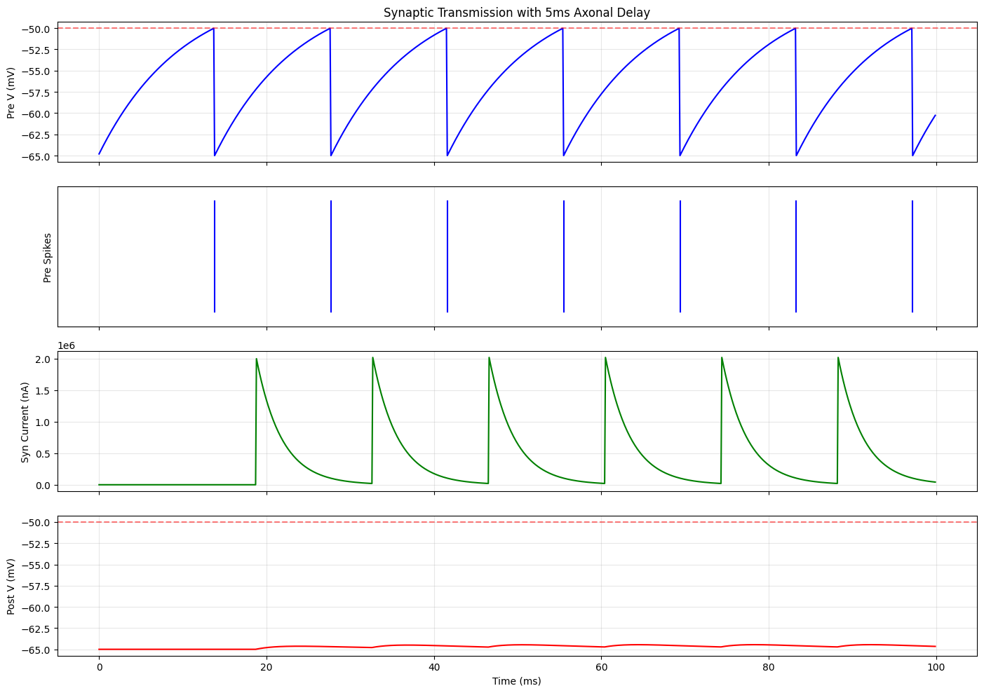
✅ Delayed synaptic transmission: presynaptic spikes appear at postsynaptic neuron after 5ms delay
   First pre spike: ~13.8ms
   First syn current rise: ~18.8ms (5ms delay)

---

Part 6: Advanced - Heterogeneous Delays

6.1 Vector Delays

BrainState supports heterogeneous delays where each element can have a different delay time:

# Create delay buffer for 3 neurons
delay_buffer = brainstate.nn.Delay(
    target_info=jnp.zeros(3),
    time=10.0 * u.ms,
)

# Register heterogeneous delays: different delay for each neuron
# Delays: [2ms, 5ms, 8ms]
delay_times = jnp.array([2.0, 5.0, 8.0]) * u.ms
neuron_indices = jnp.array([0, 1, 2])  # Which neuron

delay_buffer.register_entry('heterogeneous', delay_times, neuron_indices)
delay_buffer.init_state()

# Simulate
for i in range(200):
    brainstate.environ.set(i=i)
    
    # Update with [i, i*10, i*100]
    values = jnp.array([float(i), float(i*10), float(i*100)])
    delay_buffer.update(values)

# Retrieve heterogeneous delays
delayed_values = delay_buffer.at('heterogeneous')

expected_delays_steps = jnp.array([20, 50, 80])  # in steps (0.1ms each)
expected_values = jnp.array([
    199 - 20,
    (199 - 50) * 10,
    (199 - 80) * 100
])

print("Heterogeneous delays at step 199:")
print(f"  Delays: [2ms, 5ms, 8ms] = {expected_delays_steps} steps")
print(f"  Retrieved values: {delayed_values}")
print(f"  Expected values:  {expected_values}")
print(f"  Match: {jnp.allclose(delayed_values, expected_values)}")

print("\n✅ Vector delays enable different delay times for each element")

Heterogeneous delays at step 199:
  Delays: [2ms, 5ms, 8ms] = [20 50 80] steps
  Retrieved values: [  179.  1490. 11900.]
  Expected values:  [  179  1490 11900]
  Match: True

✅ Vector delays enable different delay times for each element

---

Summary

Key Concepts

1. brainstate.nn.Delay: General-purpose delay buffer

   • Stores rolling history of values

   • Supports rotation (ring buffer) or concatenation methods

   • Multiple named delay entries via register_entry()

   • Step-based (retrieve_at_step) or time-based (retrieve_at_time) retrieval

   • Linear or round interpolation for continuous-time queries

2. brainstate.nn.DelayAccess: Named accessor for delay entries

   • Created via delay.access(entry, delay_time)

   • Encapsulates delay configuration

   • Useful for modular design

   • Call .update() to retrieve delayed value

3. brainstate.nn.StateWithDelay: Automatic state tracking

   • Bound to a module’s State variable

   • Created via prefetch_delay(state_name, delay_time)

   • Automatically updates after each step

   • Ideal for delayed feedback and recurrent connections

   • Call as function () to retrieve delayed state

API Comparison Table

Feature	Delay	DelayAccess	StateWithDelay
Use Case	General data buffering	Named accessors	Module state tracking
Creation	Manual instantiation	Via delay.access()	Via prefetch_delay()
Updates	Manual update(value)	Inherits from Delay	Automatic after step
Retrieval	at(entry) or retrieve_at_*	.update()	Call as function ()
Multiple delays	✅ Multiple entries	✅ One per accessor	✅ Multiple registrations
Interpolation	✅ Linear or round	✅ Via underlying Delay	✅ Via underlying Delay

Best Practices

1. Choose the right tool:

   • Use Delay for general data buffering (synaptic inputs, external signals)

   • Use DelayAccess when passing delay accessors to other modules

   • Use StateWithDelay (via prefetch_delay()) for module state feedback

2. Delay method selection:

   • Default to rotation (ring buffer) for efficiency

   • Use concat only if you need sequential buffer structure

3. Interpolation:

   • Use linear_interp for smooth continuous-time delays

   • Use round for discrete time steps

4. Buffer sizing:

   • Set time parameter larger than maximum expected delay

   • Buffer size = ceil(max_delay / dt) + 1 steps

5. Initialization:

   • Always call .init_state() before simulation

   • Provide meaningful init values for t < 0 history

Common Patterns

Pattern 1: Delayed synaptic connection

# In synapse __init__:
self.spike_delay = brainstate.nn.Delay(jnp.zeros(pre_size), time=delay_time)
self.spike_delay.register_entry('syn', delay_time)

# In synapse update:
self.spike_delay.update(pre_spike)
delayed_spike = self.spike_delay.at('syn')

Pattern 2: Delayed feedback

# In neuron __init__:
self.V_delayed = self.prefetch_delay('V', feedback_delay)

# In neuron update:
V_past = self.V_delayed()
feedback = compute_feedback(V_past)

Pattern 3: Multiple delay taps

delay = brainstate.nn.Delay(data, time=max_delay)
delay.register_entry('short', 2.0 * u.ms)
delay.register_entry('medium', 5.0 * u.ms)
delay.register_entry('long', 10.0 * u.ms)

---

Exercise

Challenge: Implement a network of 3 LIF neurons with the following connections:

• Neuron 0 → Neuron 1 (2ms delay, weight=1.0)

• Neuron 1 → Neuron 2 (5ms delay, weight=1.5)

• Neuron 2 → Neuron 0 (3ms delay, weight=-0.5, inhibitory)

Use brainstate.nn.Delay for the synaptic connections and simulate for 200ms.

Hints:

1. Create 3 SimpleLIF neurons

2. Create 3 DelayedSynapse objects for the connections

3. Drive Neuron 0 with external input

4. Plot voltage traces of all 3 neurons

5. Observe the sequential activation with delays

---

What’s Next?

• Tutorial 7: Collective Operations - Learn about communication patterns in neural populations

• Advanced Delays - Explore plastic delays and state-dependent delays

• Network Architecture - Build large-scale networks with distributed delays

---

Congratulations! You now understand BrainState’s powerful delay mechanisms for modeling realistic neural dynamics. 🎉