Lifted Transforms and High-Level Optimizers

In the previous tutorial, we learned about the functional API with explicit state management using graph operations. While powerful, that approach requires manual state handling. This tutorial introduces lifted transforms - a higher-level API that automatically manages states while preserving JAX’s functional programming benefits.

Learning Objectives

By the end of this tutorial, you will:

• Understand the difference between functional API and lifted transforms

• Use BrainTools optimizers for automatic state management

• Leverage brainstate.transform for state-aware JAX transformations

• Build cleaner training loops with less boilerplate code

• Apply the lifted API to the same polynomial regression problem

Setup and Imports

import jax
import jax.numpy as jnp
import matplotlib.pyplot as plt
import numpy as np

import brainstate
import braintools

# Set random seed for reproducibility
np.random.seed(42)

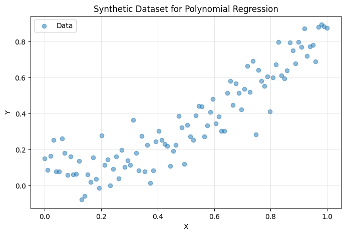
The Same Problem: Polynomial Regression

We’ll use the same dataset as the previous tutorial to highlight the differences in approach:

# Generate synthetic data: y = 0.8 * x^2 + 0.1 + noise
X = np.linspace(0, 1, 100)[:, None]
Y = 0.8 * X ** 2 + 0.1 + np.random.normal(0, 0.1, size=X.shape)

def dataset(batch_size):
    """Generator that yields random batches from the dataset."""
    while True:
        idx = np.random.choice(len(X), size=batch_size)
        yield X[idx], Y[idx]

# Visualize the data
plt.figure(figsize=(8, 5))
plt.scatter(X, Y, alpha=0.5, label='Data')
plt.xlabel('X')
plt.ylabel('Y')
plt.title('Synthetic Dataset for Polynomial Regression')
plt.legend()
plt.grid(True, alpha=0.3)
plt.show()

Building the Model with Lifted Transforms

Step 1: Define the Model Components

The model definition is similar, but we’ll use it differently:

class Linear(brainstate.nn.Module):
    """A simple linear layer: y = x @ w + b"""
    
    def __init__(self, din: int, dout: int):
        super().__init__()
        self.w = brainstate.ParamState(brainstate.random.rand(din, dout))
        self.b = brainstate.ParamState(jnp.zeros((dout,)))
    
    def __call__(self, x):
        return x @ self.w.value + self.b.value


class Count(brainstate.State):
    """Custom state type for tracking function calls."""
    pass


class MLP(brainstate.nn.Module):
    """Multi-layer perceptron with call counting.
    
    Note: Now inherits from nn.Module instead of graph.Node.
    This enables automatic state management.
    """
    
    def __init__(self, din, dhidden, dout):
        super().__init__()  # Important: call parent __init__
        
        self.count = Count(jnp.array(0))
        self.linear1 = Linear(din, dhidden)
        self.linear2 = Linear(dhidden, dout)
    
    def __call__(self, x):
        self.count.value += 1
        x = self.linear1(x)
        x = jax.nn.relu(x)
        x = self.linear2(x)
        return x

Step 2: Create Model and Optimizer

Now we create the model and use a BrainTools optimizer that automatically manages parameter states:

# Create the model
model = MLP(din=1, dhidden=32, dout=1)

# Create optimizer and register trainable weights
optimizer = braintools.optim.SGD(lr=1e-3)
optimizer.register_trainable_weights(model.states(brainstate.ParamState))

print("Model created:")
print(model)
print("\nOptimizer registered with parameters:")
print(jax.tree.map(jnp.shape, optimizer.param_states.to_pytree()))

Model created:
MLP(
  count=Count(
    value=ShapedArray(int32[], weak_type=True)
  ),
  linear1=Linear(
    w=ParamState(
      value=ShapedArray(float32[1,32])
    ),
    b=ParamState(
      value=ShapedArray(float32[32])
    )
  ),
  linear2=Linear(
    w=ParamState(
      value=ShapedArray(float32[32,1])
    ),
    b=ParamState(
      value=ShapedArray(float32[1])
    )
  )
)

Optimizer registered with parameters:
{('linear1', 'b'): (), ('linear1', 'w'): (), ('linear2', 'b'): (), ('linear2', 'w'): ()}

Key Differences from Functional API:

1. No Manual State Splitting: We don’t need to call treefy_split - the model and optimizer manage states internally

2. Optimizer Handles Parameters: The optimizer automatically tracks and updates parameters

3. Simpler Code: Less boilerplate, more readable

Training with Lifted Transforms

Understanding Lifted Transforms

Lifted transforms automatically handle state management:

• brainstate.transform.jit: JIT compilation with automatic state threading

• brainstate.transform.grad: Gradients with automatic state differentiation

• States are implicitly updated during function execution

Step 1: Define Training Step

@brainstate.transform.jit
def train_step(batch):
    """Perform one training step.
    
    Notice how much simpler this is compared to the functional API!
    No need to pass/return states explicitly.
    """
    x, y = batch
    
    def loss_fn():
        # Simply call the model - states are managed automatically
        return jnp.mean((y - model(x)) ** 2)
    
    # Compute gradients
    # The grad transform knows which states to differentiate
    grads = brainstate.transform.grad(
        loss_fn, 
        optimizer.param_states.to_pytree()
    )()
    
    # Update parameters using the optimizer
    optimizer.update(grads)

Compare with Functional API:

Functional API (previous tutorial):

def train_step(params, counts, batch):
    x, y = batch
    def loss_fn(params):
        model = brainstate.graph.treefy_merge(graphdef, params, counts)
        y_pred = model(x)
        new_counts = brainstate.graph.treefy_states(model, Count)
        loss = jnp.mean((y - y_pred) ** 2)
        return loss, new_counts
    grad, counts = jax.grad(loss_fn, has_aux=True)(params)
    params = jax.tree.map(lambda w, g: w - 0.1 * g, params, grad)
    return params, counts

Lifted API (this tutorial):

def train_step(batch):
    x, y = batch
    def loss_fn():
        return jnp.mean((y - model(x)) ** 2)
    grads = brainstate.transform.grad(loss_fn, optimizer.param_states.to_pytree())()
    optimizer.update(grads)

Much cleaner!

Step 2: Define Evaluation Step

@brainstate.transform.jit
def eval_step(batch):
    """Evaluate the model on a batch."""
    x, y = batch
    y_pred = model(x)
    loss = jnp.mean((y - y_pred) ** 2)
    return {'loss': loss}

Step 3: Run Training

# Training parameters
total_steps = 10_000

# Training loop - notice how clean this is!
print("Training the model...\n")
for step, batch in enumerate(dataset(32)):
    # Simply call train_step - no state management needed!
    train_step(batch)
    
    # Log progress every 1000 steps
    if step % 1000 == 0:
        logs = eval_step((X, Y))
        print(f"Step: {step:5d}, Loss: {logs['loss']:.6f}")
    
    # Stop after total_steps
    if step >= total_steps - 1:
        break

print("\nTraining complete!")

Training the model...

Step:     0, Loss: 17.077118
Step:  1000, Loss: 0.050319
Step:  2000, Loss: 0.018055
Step:  3000, Loss: 0.010365
Step:  4000, Loss: 0.008487
Step:  5000, Loss: 0.007985
Step:  6000, Loss: 0.007841
Step:  7000, Loss: 0.007793
Step:  8000, Loss: 0.007769
Step:  9000, Loss: 0.007754

Training complete!

Compare Training Loops:

Functional API:

for step, batch in enumerate(dataset(32)):
    params_, counts_ = train_step(params_, counts_, batch)  # Manual state threading
    if step % 1000 == 0:
        logs = eval_step(params_, counts_, (X, Y))  # Pass states explicitly

Lifted API:

for step, batch in enumerate(dataset(32)):
    train_step(batch)  # States handled automatically
    if step % 1000 == 0:
        logs = eval_step((X, Y))  # No state arguments needed

Analyzing Results

# The model already contains the trained parameters!
# No need to merge states like in functional API

print(f"Total model calls during training: {model.count.value}")

# Make predictions
y_pred = model(X)

print(f"Final predictions shape: {y_pred.shape}")

Total model calls during training: 10010
Final predictions shape: (100, 1)

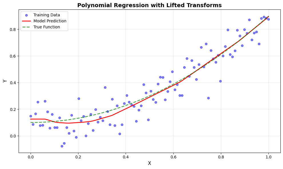
Visualize Predictions

plt.figure(figsize=(10, 6))

# Plot data points
plt.scatter(X, Y, color='blue', alpha=0.5, label='Training Data', s=30)

# Plot predictions
plt.plot(X, y_pred, color='red', linewidth=2, label='Model Prediction')

# Plot true function
X_true = np.linspace(0, 1, 100)[:, None]
Y_true = 0.8 * X_true ** 2 + 0.1
plt.plot(X_true, Y_true, color='green', linewidth=2, 
         linestyle='--', label='True Function', alpha=0.7)

plt.xlabel('X', fontsize=12)
plt.ylabel('Y', fontsize=12)
plt.title('Polynomial Regression with Lifted Transforms', fontsize=14, fontweight='bold')
plt.legend(fontsize=10)
plt.grid(True, alpha=0.3)
plt.tight_layout()
plt.show()

Advanced: Using Different Optimizers

BrainTools provides many optimizers. Let’s try Adam optimizer with learning rate scheduling:

# Create a new model
brainstate.random.seed(0)
model_adam = MLP(din=1, dhidden=32, dout=1)

# Create Adam optimizer with exponential decay learning rate
lr_schedule = braintools.optim.ExponentialDecayLR(
    1e-2,           # Initial learning rate
    decay_steps=100,   # Decay every 100 steps
    decay_rate=0.99    # Multiply by 0.99 each decay
)

optimizer_adam = braintools.optim.Adam(lr=lr_schedule)
optimizer_adam.register_trainable_weights(model_adam.states(brainstate.ParamState))

print("Adam optimizer created with learning rate scheduling!")

Adam optimizer created with learning rate scheduling!

# Define training step with the new optimizer
@brainstate.transform.jit
def train_step_adam(batch):
    x, y = batch
    
    def loss_fn():
        return jnp.mean((y - model_adam(x)) ** 2)
    
    grads = brainstate.transform.grad(
        loss_fn, 
        optimizer_adam.param_states.to_pytree()
    )()
    
    optimizer_adam.update(grads)

@brainstate.transform.jit
def eval_step_adam(batch):
    x, y = batch
    y_pred = model_adam(x)
    loss = jnp.mean((y - y_pred) ** 2)
    return {'loss': loss}

# Training with Adam
total_steps = 5_000

print("Training with Adam optimizer...\n")
for step, batch in enumerate(dataset(32)):
    train_step_adam(batch)
    
    if step % 500 == 0:
        logs = eval_step_adam((X, Y))
        current_lr = optimizer_adam.current_lr
        print(f"Step: {step:5d}, Loss: {logs['loss']:.6f}, LR: {current_lr:.6f}")
    
    if step >= total_steps - 1:
        break

print("\nTraining complete!")

Training with Adam optimizer...

Step:     0, Loss: 5.806739, LR: 0.010000
Step:   500, Loss: 0.007895, LR: 0.010000
Step:  1000, Loss: 0.007700, LR: 0.010000
Step:  1500, Loss: 0.007669, LR: 0.010000
Step:  2000, Loss: 0.007656, LR: 0.010000
Step:  2500, Loss: 0.007796, LR: 0.010000
Step:  3000, Loss: 0.007845, LR: 0.010000
Step:  3500, Loss: 0.007663, LR: 0.010000
Step:  4000, Loss: 0.007980, LR: 0.010000
Step:  4500, Loss: 0.007653, LR: 0.010000

Training complete!

Comparison: Functional API vs Lifted Transforms

Aspect	Functional API	Lifted Transforms
State Management	Manual (explicit split/merge)	Automatic (implicit)
Code Complexity	Higher (more boilerplate)	Lower (cleaner code)
Control	Full control over states	Managed by framework
Learning Curve	Steeper (need to understand graph ops)	Gentler (similar to PyTorch)
Use Cases	Custom algorithms, research	Standard training, production
Performance	Same (both compile to XLA)	Same (both compile to XLA)
Debugging	Easier to trace states	Harder (implicit state flow)
Flexibility	Maximum	High (sufficient for most cases)

When to Use Each?

Use Functional API when:

• Implementing novel optimization algorithms

• Need fine-grained control over state updates

• Debugging complex state interactions

• Research requiring custom gradient computations

Use Lifted Transforms when:

• Standard training workflows

• Production deployments

• Rapid prototyping

• When code readability is priority

Key Concepts Summary

Lifted Transforms

1. Automatic State Management:

   • States are implicitly threaded through computations

   • No need for manual split/merge operations

   • Cleaner, more readable code

2. BrainTools Optimizers:

   • Handle parameter registration and updates

   • Support learning rate scheduling

   • Implement various algorithms (SGD, Adam, AdamW, etc.)

3. BrainState Transforms:

   • brainstate.transform.jit: JIT compilation with state handling

   • brainstate.transform.grad: Gradients with automatic state differentiation

   • brainstate.transform.for_loop: Efficient loops over sequences

Best Practices

1. Start with Lifted API: Begin with lifted transforms for most projects

2. Use BrainTools Optimizers: They handle state management for you

3. Drop to Functional API when needed: For advanced control

4. Profile before optimizing: Both APIs have same performance

Exercises

Try these exercises to deepen your understanding:

1. Experiment with Optimizers:

   • Try different optimizers (AdamW, RMSprop)

   • Compare convergence speeds

   • Visualize learning curves

2. Add Regularization:

   • Implement L2 regularization in the loss function

   • Add dropout layers to the MLP

   • Compare generalization performance

3. Learning Rate Scheduling:

   • Implement cosine annealing schedule

   • Try step decay

   • Plot learning rate vs. step

4. Gradient Clipping:

   • Add gradient clipping to prevent exploding gradients

   • Monitor gradient norms during training

Next Steps

Now that you understand both functional and lifted APIs, you can:

1. Build Complex Models: Apply these concepts to CNNs, RNNs, and Transformers

2. Explore Advanced Training: Learn about mixed precision, gradient accumulation

3. Dive into Brain Models: Use these techniques for spiking neural networks

4. Checkpointing and Deployment: Save and load trained models

References

• BrainState Transform API

• BrainTools Optimizers

• JAX Documentation