
Basic Neural Network Layers#
BrainState provides a comprehensive set of pre-built layers for building neural networks. This tutorial covers the essential building blocks.
You will learn about:
📏 Linear layers - Fully connected transformations
🔲 Convolutional layers - Spatial feature extraction (1D, 2D, 3D)
🏊 Pooling layers - Downsampling operations
💧 Dropout layers - Regularization techniques
🔧 Utility layers - Flatten, reshape, and more
These layers are optimized, well-tested, and ready to use in your models!
import brainstate
from brainstate import environ
import brainunit as u
import jax.numpy as jnp
import matplotlib.pyplot as plt
import numpy as np
1. Linear (Fully Connected) Layers#
Linear layers perform the transformation: y = Wx + b.
BrainState linear modules expect feature shapes as tuples so they can validate tensor shapes. For example, use Linear(in_size=(10,), out_size=(5,)).
Basic Usage#
# Create a linear layer
brainstate.random.seed(42)
linear = brainstate.nn.Linear(in_size=(10,), out_size=(5,))

print("Linear Layer:")
print(linear)
print(f"Weight shape: {linear.weight.value['weight'].shape}")
print(f"Bias shape: {linear.weight.value['bias'].shape}")

# Forward pass
x = brainstate.random.randn(10)
y = linear(x)

print(f"Input shape: {x.shape}")
print(f"Output shape: {y.shape}")
print(f"Output: {y}")
Linear Layer:
Linear(
  in_size=(10,),
  out_size=(5,),
  w_mask=None,
  weight=ParamState(
    value={
      'bias': ShapedArray(float32[5]),
      'weight': ShapedArray(float32[10,5])
    }
  )
)
Weight shape: (10, 5)
Bias shape: (5,)
Input shape: (10,)
Output shape: (5,)
Output: [ 0.24681929  1.2860886  -1.6367221   0.29457197 -0.9486235 ]
Batch Processing#
Linear layers automatically handle batched inputs:
# Batched input: (batch_size, features)
x_batch = brainstate.random.randn(32, 10)  # 32 samples, 10 features each
y_batch = linear(x_batch)

print(f"Batched input shape: {x_batch.shape}")
print(f"Batched output shape: {y_batch.shape}")

# Works with arbitrary batch dimensions
x_multi = brainstate.random.randn(8, 4, 10)  # (batch1, batch2, features)
y_multi = linear(x_multi)

print(f"\nMulti-batch input: {x_multi.shape}")
print(f"Multi-batch output: {y_multi.shape}")
Batched input shape: (32, 10)
Batched output shape: (32, 5)

Multi-batch input: (8, 4, 10)
Multi-batch output: (8, 4, 5)
Linear Layer Variants#
BrainState provides specialized linear layers:
ScaledWSLinearapplies weight standardization for stable training.LoRAadds low-rank adapters to an existing projection.SparseLinearconsumes abrainunit.sparsematrix so you can encode custom connectivity patterns.
# SparseLinear: For sparse connectivity
brainstate.random.seed(0)
dense_weight = brainstate.random.rand(100, 50)
sparsity_mask = brainstate.random.rand(100, 50) < 0.1
sparse_matrix = u.sparse.CSR.fromdense(dense_weight * sparsity_mask)
sparse_linear = brainstate.nn.SparseLinear(sparse_matrix, in_size=(100,))

print("Sparse Linear Layer:")
print(sparse_linear)

x = brainstate.random.rand(100)
y = sparse_linear(x)
print(f"Input: {x.shape} → Output: {y.shape}")
Sparse Linear Layer:
SparseLinear(
  in_size=(100,),
  out_size=(50,),
  spar_mat=CSR(float32[100, 50], nse=485),
  weight=ParamState(
    value={
      'weight': ShapedArray(float32[485])
    }
  )
)
Input: (100,) → Output: (50,)
2. Convolutional Layers#
Convolutional layers extract spatial features using learnable filters. Supply the expected input shape (without the batch dimension) via in_size so each layer can initialize weights and validate its inputs.
Conv1d - 1D Convolution#
Used for sequential data (time series, audio, text):
# Conv1d: (batch, length, in_channels) → (batch, length, out_channels)
brainstate.random.seed(0)
conv1d = brainstate.nn.Conv1d(
    in_size=(100, 3),
    out_channels=16,
    kernel_size=3,
    padding='SAME'
)

print("Conv1d Layer:")
print(conv1d)

# Input: (batch=4, length=100, channels=3)
x = brainstate.random.randn(4, 100, 3)
y = conv1d(x)

print(f"Input shape: {x.shape}")
print(f"Output shape: {y.shape}")
print(f"Kernel shape: {conv1d.weight.value['weight'].shape}")
Conv1d Layer:
Conv1d(
  in_size=(100, 3),
  out_size=(100, 16),
  channel_first=False,
  channels_last=True,
  in_channels=3,
  out_channels=16,
  stride=(1,),
  kernel_size=(3,),
  lhs_dilation=(1,),
  rhs_dilation=(1,),
  groups=1,
  dimension_numbers=ConvDimensionNumbers(lhs_spec=(0, 2, 1), rhs_spec=(2, 1, 0), out_spec=(0, 2, 1)),
  padding=SAME,
  kernel_shape=(3, 3, 16),
  w_mask=None,
  w_initializer=XavierNormal(
    scale=1.0,
    mode='fan_avg',
    in_axis=-2,
    out_axis=-1,
    distribution='truncated_normal',
    rng=RandomState([1797259609 2579123966]),
    unit=Unit(10.0^0)
  ),
  b_initializer=None,
  weight=ParamState(
    value={
      'weight': ShapedArray(float32[3,3,16])
    }
  )
)
Input shape: (4, 100, 3)
Output shape: (4, 100, 16)
Kernel shape: (3, 3, 16)
Conv2d - 2D Convolution#
The workhorse for image processing:
# Conv2d: (batch, height, width, in_channels) → (batch, height, width, out_channels)
conv2d = brainstate.nn.Conv2d(
    in_size=(28, 28, 3),      # (height, width, channels)
    out_channels=32,          # 32 feature maps
    kernel_size=(3, 3),       # 3x3 kernel
    stride=(1, 1),            # Stride of 1
    padding='SAME'
)

print("Conv2d Layer:")
print(conv2d)

# Input: (batch=8, height=28, width=28, channels=3)
x_image = brainstate.random.randn(8, 28, 28, 3)
y_image = conv2d(x_image)

print(f"Input shape: {x_image.shape}")
print(f"Output shape: {y_image.shape}")
print(f"Kernel shape: {conv2d.weight.value['weight'].shape}")
Conv2d Layer:
Conv2d(
  in_size=(28, 28, 3),
  out_size=(28, 28, 32),
  channel_first=False,
  channels_last=True,
  in_channels=3,
  out_channels=32,
  stride=(1, 1),
  kernel_size=(3, 3),
  lhs_dilation=(1, 1),
  rhs_dilation=(1, 1),
  groups=1,
  dimension_numbers=ConvDimensionNumbers(lhs_spec=(0, 3, 1, 2), rhs_spec=(3, 2, 0, 1), out_spec=(0, 3, 1, 2)),
  padding=SAME,
  kernel_shape=(3, 3, 3, 32),
  w_mask=None,
  w_initializer=XavierNormal(
    scale=1.0,
    mode='fan_avg',
    in_axis=-2,
    out_axis=-1,
    distribution='truncated_normal',
    rng=RandomState([ 683029726 1624662641]),
    unit=Unit(10.0^0)
  ),
  b_initializer=None,
  weight=ParamState(
    value={
      'weight': ShapedArray(float32[3,3,3,32])
    }
  )
)
Input shape: (8, 28, 28, 3)
Output shape: (8, 28, 28, 32)
Kernel shape: (3, 3, 3, 32)
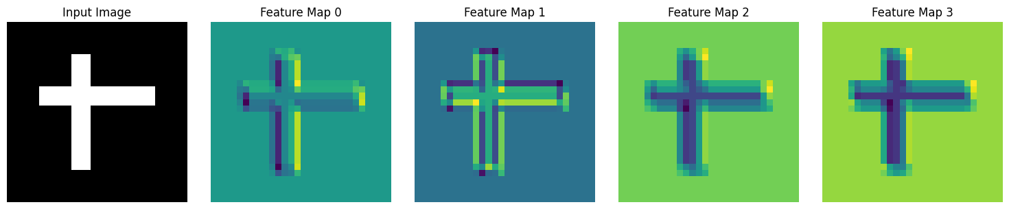
Visualizing Convolutional Features#
# Create a simple image with a pattern
def create_test_image():
    img = jnp.zeros((28, 28, 1))
    # Add vertical edge
    img = img.at[5:23, 10:13, 0].set(1.0)
    # Add horizontal edge
    img = img.at[10:13, 5:23, 0].set(1.0)
    return img

# Create and apply conv
brainstate.random.seed(42)
edge_conv = brainstate.nn.Conv2d(
    in_size=(28, 28, 1),
    out_channels=4,
    kernel_size=(3, 3),
    padding='SAME'
)

test_img = create_test_image()
features = edge_conv(test_img[None, ...])[0]  # Add/remove batch dim

# Visualize
fig, axes = plt.subplots(1, 5, figsize=(15, 3))

# Original image
axes[0].imshow(test_img[:, :, 0], cmap='gray')
axes[0].set_title('Input Image')
axes[0].axis('off')

# Feature maps
for i in range(4):
    axes[i+1].imshow(np.array(features[:, :, i]), cmap='viridis')
    axes[i+1].set_title(f'Feature Map {i}')
    axes[i+1].axis('off')

plt.tight_layout()
plt.show()
Convolution Parameters#
Understanding stride and padding (stride=..., padding=...):
stridecontrols the step size; pass it with thestridekeyword (the API no longer acceptsstrides).'SAME'padding preserves spatial dimensions when the stride is 1;'VALID'performs no padding.Explicit tuples let you set different values per spatial dimension.
# Different stride values
x = brainstate.random.randn(1, 28, 28, 3)

configs = [
    {'stride': (1, 1), 'padding': 'SAME', 'name': 'Stride 1, SAME'},
    {'stride': (2, 2), 'padding': 'SAME', 'name': 'Stride 2, SAME'},
    {'stride': (1, 1), 'padding': 'VALID', 'name': 'Stride 1, VALID'},
]

print(f"Input shape: {x.shape}")

for config in configs:
    brainstate.random.seed(0)
    conv = brainstate.nn.Conv2d(
        in_size=(28, 28, 3),
        out_channels=16,
        kernel_size=(3, 3),
        stride=config['stride'],
        padding=config['padding']
    )
    y = conv(x)
    print(f"{config['name']:20s}: {y.shape}")
Input shape: (1, 28, 28, 3)
Stride 1, SAME      : (1, 28, 28, 16)
Stride 2, SAME      : (1, 14, 14, 16)
Stride 1, VALID     : (1, 26, 26, 16)
Conv3d - 3D Convolution#
For video or volumetric data:
# Conv3d: (batch, depth, height, width, channels)
conv3d = brainstate.nn.Conv3d(
    in_size=(16, 64, 64, 3),
    out_channels=16,
    kernel_size=(3, 3, 3),
    padding='SAME'
)

# Video input: (batch=2, frames=16, height=64, width=64, channels=3)
x_video = brainstate.random.randn(2, 16, 64, 64, 3)
y_video = conv3d(x_video)

print(f"Video input shape: {x_video.shape}")
print(f"Video output shape: {y_video.shape}")
Video input shape: (2, 16, 64, 64, 3)
Video output shape: (2, 16, 64, 64, 16)
3. Pooling Layers#
Pooling layers downsample feature maps, reducing spatial dimensions.
Max Pooling#
# MaxPool2d: Takes maximum value in each window
maxpool = brainstate.nn.MaxPool2d(
    kernel_size=(2, 2),
    stride=(2, 2)
)

print("MaxPool2d Layer:")
print(maxpool)

# Input: (batch=4, height=28, width=28, channels=16)
x = brainstate.random.randn(4, 28, 28, 16)
y = maxpool(x)

print(f"Input shape: {x.shape}")
print(f"Output shape: {y.shape}")
print(f"Spatial reduction: {x.shape[1]}x{x.shape[2]} → {y.shape[1]}x{y.shape[2]}")
MaxPool2d Layer:
MaxPool2d(
  init_value=-inf,
  computation=<function max at 0x00000207E9544220>,
  pool_dim=2,
  return_indices=False,
  kernel_size=(2, 2),
  stride=(2, 2),
  padding=VALID,
  channel_axis=-1
)
Input shape: (4, 28, 28, 16)
Output shape: (4, 14, 14, 16)
Spatial reduction: 28x28 → 14x14
Average Pooling#
# AvgPool2d: Takes average value in each window
avgpool = brainstate.nn.AvgPool2d(
    kernel_size=(2, 2),
    stride=(2, 2)
)

y_avg = avgpool(x)

print("AvgPool2d Layer:")
print(avgpool)
print(f"Output shape: {y_avg.shape}")
AvgPool2d Layer:
AvgPool2d(
  init_value=0.0,
  computation=<function add at 0x00000207E9587EC0>,
  pool_dim=2,
  return_indices=False,
  kernel_size=(2, 2),
  stride=(2, 2),
  padding=VALID,
  channel_axis=-1
)
Output shape: (4, 14, 14, 16)
Adaptive Pooling#
Pools to a fixed output size regardless of input size:
# AdaptiveAvgPool2d: Always outputs specified size
adaptive_pool = brainstate.nn.AdaptiveAvgPool2d(target_size=(7, 7))

# Works with any input size
inputs = [
    brainstate.random.randn(1, 28, 28, 16),
    brainstate.random.randn(1, 56, 56, 16),
    brainstate.random.randn(1, 224, 224, 16),
]

print("AdaptiveAvgPool2d (output: 7x7)")
for i, x in enumerate(inputs):
    y = adaptive_pool(x)
    print(f"Input {x.shape[1:3]} → Output {y.shape[1:3]}")
AdaptiveAvgPool2d (output: 7x7)
Input (28, 28) → Output (7, 7)
Input (56, 56) → Output (7, 7)
Input (224, 224) → Output (7, 7)
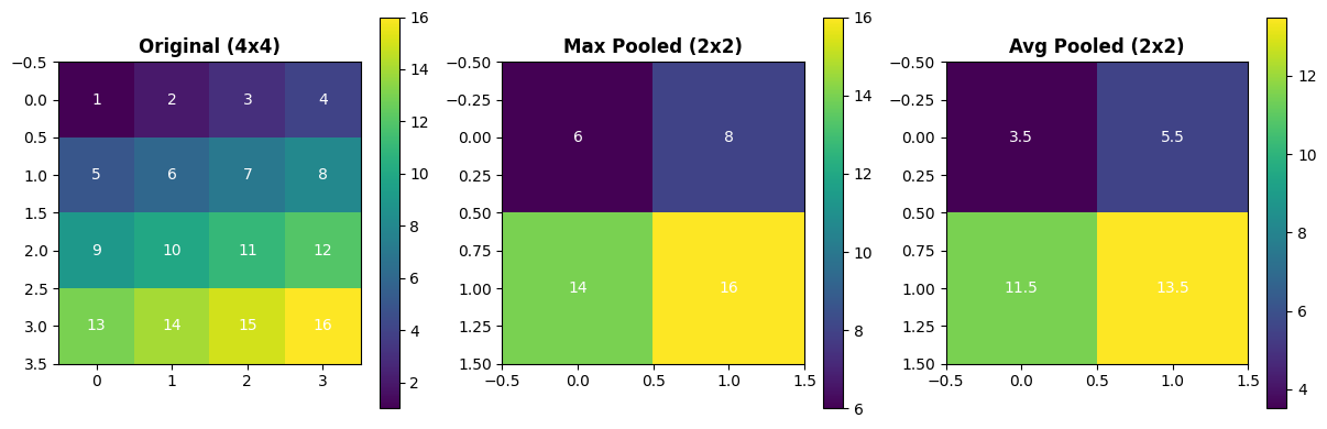
Comparing Pooling Operations#
# Create a simple test pattern
x_test = jnp.array([
    [1, 2, 3, 4],
    [5, 6, 7, 8],
    [9, 10, 11, 12],
    [13, 14, 15, 16]
], dtype=jnp.float32)

x_test = x_test[None, :, :, None]  # Add batch and channel dims

# Apply different pooling
maxpool_2x2 = brainstate.nn.MaxPool2d(kernel_size=(2, 2), stride=(2, 2))
avgpool_2x2 = brainstate.nn.AvgPool2d(kernel_size=(2, 2), stride=(2, 2))

y_max = maxpool_2x2(x_test)
y_avg = avgpool_2x2(x_test)

fig, axes = plt.subplots(1, 3, figsize=(12, 4))

# Original
im1 = axes[0].imshow(x_test[0, :, :, 0], cmap='viridis', interpolation='nearest')
axes[0].set_title('Original (4x4)', fontsize=12, fontweight='bold')
for i in range(4):
    for j in range(4):
        axes[0].text(j, i, f'{x_test[0,i,j,0]:.0f}',
                    ha='center', va='center', color='white', fontsize=10)
plt.colorbar(im1, ax=axes[0])

# Max pooled
im2 = axes[1].imshow(y_max[0, :, :, 0], cmap='viridis', interpolation='nearest')
axes[1].set_title('Max Pooled (2x2)', fontsize=12, fontweight='bold')
for i in range(2):
    for j in range(2):
        axes[1].text(j, i, f'{y_max[0,i,j,0]:.0f}',
                    ha='center', va='center', color='white', fontsize=10)
plt.colorbar(im2, ax=axes[1])

# Avg pooled
im3 = axes[2].imshow(y_avg[0, :, :, 0], cmap='viridis', interpolation='nearest')
axes[2].set_title('Avg Pooled (2x2)', fontsize=12, fontweight='bold')
for i in range(2):
    for j in range(2):
        axes[2].text(j, i, f'{y_avg[0,i,j,0]:.1f}',
                    ha='center', va='center', color='white', fontsize=10)
plt.colorbar(im3, ax=axes[2])

plt.tight_layout()
plt.show()

print("MaxPool takes the maximum value from each 2x2 window")
print("AvgPool takes the average value from each 2x2 window")
MaxPool takes the maximum value from each 2x2 window
AvgPool takes the average value from each 2x2 window
4. Dropout and Regularization#
Dropout randomly sets activations to zero during training for regularization. Pass prob to control the keep probability and enable stochastic behaviour with environ.context(fit=True) during training.
Standard Dropout#
# Dropout: Randomly zero out elements
dropout = brainstate.nn.Dropout(prob=0.5)  # Keep 50% of activations during training

print("Dropout Layer:")
print(dropout)

# Create test input
brainstate.random.seed(42)
x = jnp.ones(10)

print("Original:", x)
print("Dropout outputs (training mode):")
with environ.context(fit=True):
    for i in range(3):
        y = dropout(x)
        print(f"  {i + 1}: {y}")

with environ.context(fit=False):
    stable = dropout(x)

print("Evaluation mode:", stable)
Dropout Layer:
Dropout(
  prob=0.5,
  broadcast_dims=()
)
Original: [1. 1. 1. 1. 1. 1. 1. 1. 1. 1.]
Dropout outputs (training mode):
  1: [0. 0. 2. 2. 2. 2. 2. 2. 2. 2.]
  2: [2. 2. 2. 2. 0. 2. 0. 0. 0. 2.]
  3: [2. 2. 2. 2. 0. 0. 2. 0. 0. 0.]
Evaluation mode: [1. 1. 1. 1. 1. 1. 1. 1. 1. 1.]
Training vs Evaluation Mode#
Dropout behaves differently during training and evaluation:
Wrap forward passes in
with environ.context(fit=True):to enable dropout.Outside that context (or with
fit=False) dropout becomes a no-op for deterministic evaluation.
class NetworkWithDropout(brainstate.nn.Module):
    def __init__(self, input_dim, hidden_dim, output_dim):
        super().__init__()
        self.linear1 = brainstate.nn.Linear((input_dim,), (hidden_dim,))
        self.dropout = brainstate.nn.Dropout(prob=0.5)
        self.linear2 = brainstate.nn.Linear((hidden_dim,), (output_dim,))

    def update(self, x):
        x = self.linear1(x)
        x = jnp.maximum(0, x)  # ReLU
        x = self.dropout(x)
        x = self.linear2(x)
        return x

# Create network
brainstate.random.seed(0)
net = NetworkWithDropout(10, 20, 5)

# Test input
x = brainstate.random.randn(10)

# Compare outputs in training mode
with environ.context(fit=True):
    y1 = net(x)
    y2 = net(x)

with environ.context(fit=False):
    y_eval = net(x)

print("With dropout (training):")
print(f"  Output 1: {y1}")
print(f"  Output 2: {y2}")
print(f"  Outputs differ: {not jnp.allclose(y1, y2)}")

print("Evaluation mode (dropout off):")
print(f"  Output: {y_eval}")
With dropout (training):
  Output 1: [ 1.7709473  -1.7486901  -0.11733629  0.30774632  1.7717932 ]
  Output 2: [-2.4300232   0.03660802  1.8875287  -1.3981102  -0.3061459 ]
  Outputs differ: True
Evaluation mode (dropout off):
  Output: [-0.44592363 -0.25877538  0.6993926  -1.0398884   0.14154091]
5. Utility Layers#
Flatten Layer#
Flattens multi-dimensional inputs:
# Flatten: Reshape to 1D
flatten = brainstate.nn.Flatten(start_axis=1)

# Example: After convolution, flatten before fully connected
x_conv = brainstate.random.randn(4, 7, 7, 64)  # (batch, H, W, C)
x_flat = flatten(x_conv)

print(f"Before flatten: {x_conv.shape}")
print(f"After flatten: {x_flat.shape}")
print(f"Flattened: {7 * 7 * 64} = {x_flat.shape[1]} features per sample")
Before flatten: (4, 7, 7, 64)
After flatten: (4, 3136)
Flattened: 3136 = 3136 features per sample
6. Building a Complete CNN#
Let’s combine everything into a complete convolutional neural network:
class SimpleCNN(brainstate.nn.Module):
    'Simple CNN for image classification.'

    def __init__(self, num_classes=10):
        super().__init__()

        # Conv block 1
        self.conv1 = brainstate.nn.Conv2d((32, 32, 3), out_channels=32, kernel_size=(3, 3), padding='SAME')
        self.pool1 = brainstate.nn.MaxPool2d(kernel_size=(2, 2), stride=(2, 2))

        # Conv block 2
        self.conv2 = brainstate.nn.Conv2d((16, 16, 32), out_channels=64, kernel_size=(3, 3), padding='SAME')
        self.pool2 = brainstate.nn.MaxPool2d(kernel_size=(2, 2), stride=(2, 2))

        # Conv block 3
        self.conv3 = brainstate.nn.Conv2d((8, 8, 64), out_channels=128, kernel_size=(3, 3), padding='SAME')
        self.pool3 = brainstate.nn.MaxPool2d(kernel_size=(2, 2), stride=(2, 2), in_size=self.conv3.out_size)

        # Flatten and classify
        self.flatten = brainstate.nn.Flatten(in_size=self.pool3.out_size)
        self.fc1 = brainstate.nn.Linear(4 * 4 * 128, (256,))  # Assuming 32x32 input
        self.dropout = brainstate.nn.Dropout(prob=0.5)
        self.fc2 = brainstate.nn.Linear((256,), (num_classes,))

    def update(self, x):
        # Conv block 1
        x = self.conv1(x)
        x = jnp.maximum(0, x)  # ReLU
        x = self.pool1(x)

        # Conv block 2
        x = self.conv2(x)
        x = jnp.maximum(0, x)
        x = self.pool2(x)

        # Conv block 3
        x = self.conv3(x)
        x = jnp.maximum(0, x)
        x = self.pool3(x)

        # Classifier
        x = self.flatten(x)
        x = self.fc1(x)
        x = jnp.maximum(0, x)
        x = self.dropout(x)
        x = self.fc2(x)

        return x

# Create CNN
brainstate.random.seed(42)
cnn = SimpleCNN(num_classes=10)

print("Simple CNN Architecture:")
print(cnn)

# Test with batch of images
batch_size = 8
images = brainstate.random.randn(batch_size, 32, 32, 3)  # CIFAR-10 size
with brainstate.environ.context(fit=True):
    logits = cnn(images)

print(f"Input shape: {images.shape}")
print(f"Output shape: {logits.shape}")
print(f"Logits for first image: {logits[0]}")
Simple CNN Architecture:
SimpleCNN(
  conv1=Conv2d(
    in_size=(32, 32, 3),
    out_size=(32, 32, 32),
    channel_first=False,
    channels_last=True,
    in_channels=3,
    out_channels=32,
    stride=(1, 1),
    kernel_size=(3, 3),
    lhs_dilation=(1, 1),
    rhs_dilation=(1, 1),
    groups=1,
    dimension_numbers=ConvDimensionNumbers(lhs_spec=(0, 3, 1, 2), rhs_spec=(3, 2, 0, 1), out_spec=(0, 3, 1, 2)),
    padding=SAME,
    kernel_shape=(3, 3, 3, 32),
    w_mask=None,
    w_initializer=XavierNormal(
      scale=1.0,
      mode='fan_avg',
      in_axis=-2,
      out_axis=-1,
      distribution='truncated_normal',
      rng=RandomState([ 827075891 2691092366]),
      unit=Unit(10.0^0)
    ),
    b_initializer=None,
    weight=ParamState(
      value={
        'weight': ShapedArray(float32[3,3,3,32])
      }
    )
  ),
  pool1=MaxPool2d(
    init_value=-inf,
    computation=<function max at 0x00000207E9544220>,
    pool_dim=2,
    return_indices=False,
    kernel_size=(2, 2),
    stride=(2, 2),
    padding=VALID,
    channel_axis=-1
  ),
  conv2=Conv2d(
    in_size=(16, 16, 32),
    out_size=(16, 16, 64),
    channel_first=False,
    channels_last=True,
    in_channels=32,
    out_channels=64,
    stride=(1, 1),
    kernel_size=(3, 3),
    lhs_dilation=(1, 1),
    rhs_dilation=(1, 1),
    groups=1,
    dimension_numbers=ConvDimensionNumbers(lhs_spec=(0, 3, 1, 2), rhs_spec=(3, 2, 0, 1), out_spec=(0, 3, 1, 2)),
    padding=SAME,
    kernel_shape=(3, 3, 32, 64),
    w_mask=None,
    w_initializer=XavierNormal(
      scale=1.0,
      mode='fan_avg',
      in_axis=-2,
      out_axis=-1,
      distribution='truncated_normal',
      rng=RandomState([ 827075891 2691092366]),
      unit=Unit(10.0^0)
    ),
    b_initializer=None,
    weight=ParamState(
      value={
        'weight': ShapedArray(float32[3,3,32,64])
      }
    )
  ),
  pool2=MaxPool2d(
    init_value=-inf,
    computation=<function max at 0x00000207E9544220>,
    pool_dim=2,
    return_indices=False,
    kernel_size=(2, 2),
    stride=(2, 2),
    padding=VALID,
    channel_axis=-1
  ),
  conv3=Conv2d(
    in_size=(8, 8, 64),
    out_size=(8, 8, 128),
    channel_first=False,
    channels_last=True,
    in_channels=64,
    out_channels=128,
    stride=(1, 1),
    kernel_size=(3, 3),
    lhs_dilation=(1, 1),
    rhs_dilation=(1, 1),
    groups=1,
    dimension_numbers=ConvDimensionNumbers(lhs_spec=(0, 3, 1, 2), rhs_spec=(3, 2, 0, 1), out_spec=(0, 3, 1, 2)),
    padding=SAME,
    kernel_shape=(3, 3, 64, 128),
    w_mask=None,
    w_initializer=XavierNormal(
      scale=1.0,
      mode='fan_avg',
      in_axis=-2,
      out_axis=-1,
      distribution='truncated_normal',
      rng=RandomState([ 827075891 2691092366]),
      unit=Unit(10.0^0)
    ),
    b_initializer=None,
    weight=ParamState(
      value={
        'weight': ShapedArray(float32[3,3,64,128])
      }
    )
  ),
  pool3=MaxPool2d(
    in_size=(8, 8, 128),
    out_size=(4, 4, 128),
    init_value=-inf,
    computation=<function max at 0x00000207E9544220>,
    pool_dim=2,
    return_indices=False,
    kernel_size=(2, 2),
    stride=(2, 2),
    padding=VALID,
    channel_axis=-1
  ),
  flatten=Flatten(
    in_size=(4, 4, 128),
    out_size=(2048,),
    start_axis=0,
    end_axis=-1
  ),
  fc1=Linear(
    in_size=(2048,),
    out_size=(256,),
    w_mask=None,
    weight=ParamState(
      value={
        'bias': ShapedArray(float32[256]),
        'weight': ShapedArray(float32[2048,256])
      }
    )
  ),
  dropout=Dropout(
    prob=0.5,
    broadcast_dims=()
  ),
  fc2=Linear(
    in_size=(256,),
    out_size=(10,),
    w_mask=None,
    weight=ParamState(
      value={
        'bias': ShapedArray(float32[10]),
        'weight': ShapedArray(float32[256,10])
      }
    )
  )
)
Input shape: (8, 32, 32, 3)
Output shape: (8, 10)
Logits for first image: [ 0.56677586  0.50766015  0.52835876 -0.21623717  0.56475204  0.07235158
  0.78321373 -0.7866179  -0.6562584   0.10693423]
Visualizing CNN Feature Maps#
# Get intermediate features
def get_conv_features(model, x):
    """Extract features from each conv layer."""
    features = []

    # Conv 1
    x = model.conv1(x)
    x = jnp.maximum(0, x)
    features.append(x)
    x = model.pool1(x)

    # Conv 2
    x = model.conv2(x)
    x = jnp.maximum(0, x)
    features.append(x)
    x = model.pool2(x)

    # Conv 3
    x = model.conv3(x)
    x = jnp.maximum(0, x)
    features.append(x)

    return features

# Extract features
single_image = images[0:1]  # Take first image
features = get_conv_features(cnn, single_image)

# Visualize
fig, axes = plt.subplots(1, 4, figsize=(16, 4))

# Original image
axes[0].imshow((np.array(single_image[0]) + 1) / 2)  # Normalize to [0,1]
axes[0].set_title('Input Image\n(32×32×3)', fontsize=10, fontweight='bold')
axes[0].axis('off')

# Feature maps
layer_names = ['Conv1\n(32×32×32)', 'Conv2\n(16×16×64)', 'Conv3\n(8×8×128)']
for i, (feat, name) in enumerate(zip(features, layer_names)):
    # Show first feature map from each layer
    feat_map = np.array(feat[0, :, :, 0])
    axes[i+1].imshow(feat_map, cmap='viridis')
    axes[i+1].set_title(name, fontsize=10, fontweight='bold')
    axes[i+1].axis('off')

plt.tight_layout()
plt.show()

print("Feature map shapes:")
for i, feat in enumerate(features):
    print(f"  Layer {i+1}: {feat.shape}")
Clipping input data to the valid range for imshow with RGB data ([0..1] for floats or [0..255] for integers). Got range [-1.3665657..2.0698853].
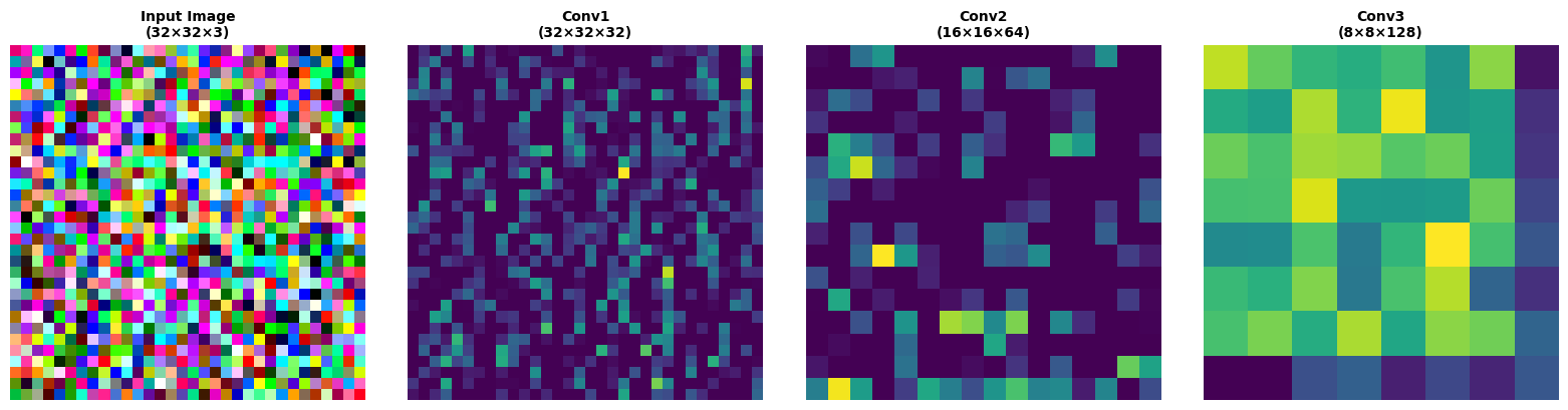
Feature map shapes:
  Layer 1: (1, 32, 32, 32)
  Layer 2: (1, 16, 16, 64)
  Layer 3: (1, 8, 8, 128)
Summary#
In this tutorial, you learned about:
✅ Linear layers - Fully connected transformations
✅ Convolutional layers - 1D, 2D, 3D spatial feature extraction
✅ Pooling layers - Max, average, and adaptive pooling
✅ Dropout - Regularization through random masking
✅ Utility layers - Flatten and reshape operations
✅ Complete CNN - Building end-to-end architectures
Key Takeaways#
Layer Type |
Use Case |
Key Parameters |
|---|---|---|
Linear |
Fully connected |
|
Conv2d |
Image features |
|
MaxPool2d |
Downsampling |
|
Dropout |
Regularization |
|
Flatten |
Shape transformation |
|
Best Practices#
🎯 Use SAME padding to preserve spatial dimensions
🧮 Provide the correct
in_sizeso layers can validate incoming tensors💧 Add dropout after dense layers for regularization
🏊 Pool after activation - standard practice in CNNs
🔍 Visualize features - helps debug and understand the network
Next Steps#
Continue with:
Activations & Normalization - Improve training stability
Recurrent Networks - Handle sequential data
Training - Put it all together with optimization