Simulation and Analysis of Excitatory-Inhibitory Neuronal Networks (E-I Networks)

This example demonstrates the implementation of a classical excitatory-inhibitory (E-I) neuronal network using the braincell framework. By constructing an E-I network composed of Hodgkin-Huxley model neurons, you will learn how to implement hierarchical modeling from single neurons to networks in braincell, and analyze the spike dynamics of the network.

Preparation

First, ensure that the necessary libraries (braincell, brainstate, brainunit, matplotlib) are installed, and import the required modules:

import brainpy
import brainunit as u
import matplotlib.pyplot as plt
import brainstate
import braincell

An NVIDIA GPU may be present on this machine, but a CUDA-enabled jaxlib is not installed. Falling back to cpu.

Code Explanation

Parameter Definition

First, define the key biophysical parameters, which determine the electrophysiological properties of the neurons and the network size:

# Neuron action potential firing threshold
V_th = -20. * u.mV

# Neuron membrane area
area = 20000 * u.um **2
area = area.in_unit(u.cm** 2)

# Membrane capacitance
Cm = (1 * u.uF * u.cm ** -2) * area  # Total capacitance = specific capacitance × area

Define HH single neuron model

Use SingleCompartment to construct a single neuron based on the HH model, including sodium channel INa, potassium channel IK, and leak current IL. These channels jointly determine the firing properties of the neuron:

class HH(braincell.SingleCompartment):
    def __init__(self, in_size):
        # Initialize single-compartment neuron
        super().__init__(in_size, C=Cm, solver='ind_exp_euler')

        # Sodium channel (INa)
        self.na = braincell.ion.SodiumFixed(in_size, E=50. * u.mV)
        self.na.add(
            # Maximum conductance
            INa=braincell.channel.Na_TM1991(in_size, g_max=(100. * u.mS * u.cm **-2) * area, V_sh=-63. * u.mV)
        )

        # Potassium channel (IK)
        self.k = braincell.ion.PotassiumFixed(in_size, E=-90 * u.mV)
        self.k.add(
            # Maximum conductance
            IK=braincell.channel.K_TM1991(in_size, g_max=(30. * u.mS * u.cm** -2) * area, V_sh=-63. * u.mV)
        )

        # Leak current (IL)
        self.IL = braincell.channel.IL(
            in_size,
            E=-60. * u.mV,
            g_max=(5. * u.nS * u.cm **-2) * area  # Maximum conductance
        )

Define E-I Network: Connections Between Excitatory and Inhibitory Neurons

Construct a network composed of excitatory (E) and inhibitory (I) neurons to simulate the commonly observed E-I balance mechanism in cortical networks:

class EINet(brainstate.nn.Module):
    def __init__(self):
        super().__init__()
        # Network scale
        self.n_exc = 3200
        self.n_inh = 800
        self.num = self.n_exc + self.n_inh  # Total number of neurons: 4000

        # Initialize neuron population
        self.N = HH(self.num)

        # Excitatory synaptic projection
        self.E = brainpy.state.AlignPostProj(
            # Connection rule
            comm=brainstate.nn.EventFixedProb(
                self.n_exc, self.num, conn_num=0.02,  # Connection probability
                conn_weight=6. * u.nS  # Synaptic weight
            ),
            # Synaptic dynamics
            syn=brainpy.state.Expon(self.num, tau=5. * u.ms),
            # Postsynaptic effect
            out=brainpy.state.COBA(E=0. * u.mV),
            post=self.N  # Projection target is neuron population N
        )

        # Inhibitory synaptic projection
        self.I = brainpy.state.AlignPostProj(
            # Connection rule
            comm=brainstate.nn.EventFixedProb(
                self.n_inh, self.num, conn_num=0.02,
                conn_weight=67. * u.nS
            ),
            # Synaptic dynamics
            syn=brainpy.state.Expon(self.num, tau=10. * u.ms),
            # Postsynaptic effect
            out=brainpy.state.COBA(E=-80. * u.mV),
            post=self.N  # Projection target is neuron population N
        )

    def update(self, t):
        # Define network update rules over time
        with brainstate.environ.context(t=t):
            # Get spike signals at current time
            spk = self.N.spike.value

            # Spikes from excitatory neurons drive excitatory synaptic projection
            self.E(spk[:self.n_exc])

            # Spikes from inhibitory neurons drive inhibitory synaptic projection
            self.I(spk[self.n_exc:])

            # Neurons update their states after receiving synaptic inputs, return new spike signals
            spk = self.N(0. * u.nA)

            return spk

Run network simulation

Initialize the network and run the simulation, recording the spike activity of neurons at each time point:

# Initialize E-I network
net = EINet()
brainstate.nn.init_all_states(net)  # Initialize the states of all neurons and synapses in the network

# Set simulation parameters and run
with brainstate.environ.context(dt=0.1 * u.ms):  # Time step
    # Generate simulation time sequence
    times = u.math.arange(0. * u.ms, 100. * u.ms, brainstate.environ.get_dt())

    # Loop to update network states
    spikes = brainstate.transform.for_loop(
        net.update, times,
        pbar=brainstate.transform.ProgressBar(10)  # Display progress bar
    )

Visualize network spike activity

Plot the spike data as a raster plot to intuitively show the firing patterns of neurons over time:

# Extract spike times and neuron indices
t_indices, n_indices = u.math.where(spikes)

# Plot raster plot
plt.scatter(times[t_indices] / u.ms, n_indices, s=1)
plt.xlabel('Time (ms)')  # X-axis: time
plt.ylabel('Neuron index')  # Y-axis: neuron index
plt.show()

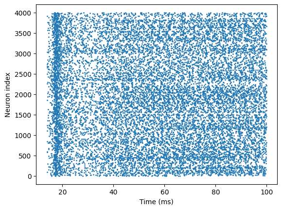
Results Interpretation

After running the code, you will see a raster plot, as shown below:

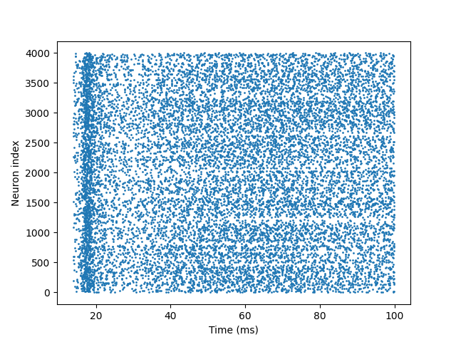
Each point represents a spike fired by a neuron at a specific time. Typical dynamics of an E-I network have the following characteristics:

• Asynchronous firing: Neurons fire at dispersed times without obvious synchronous rhythms.

• Sparse activity: Most neurons fire only a few times within 100 ms.

• No burst synchronization: Rapid feedback from inhibitory synapses prevents large-scale synchronous bursting.

These features indicate that the E-I network maintains a stable and physiologically realistic activity pattern through dynamic balance between excitatory and inhibitory neurons.

Extended Exercises

• Adjust inhibitory synaptic weights and observe whether the network exhibits excessive synchronization or bursting activity.

• Increase the proportion of excitatory neurons to analyze the impact of E-I imbalance on network dynamics.

• Extend the simulation duration to see if the network maintains stable asynchronous activity.

Through these extensions, you can gain deeper insights into the critical role of E-I balance in maintaining neural network function, and the flexibility of braincell in modeling complex networks.