Defining Differential Equations

This page shows how to express a differential-equation system in braincell using the two protocol pieces introduced in the overview: DiffEqState and DiffEqModule. By the end you will have built a runnable model from scratch and integrated it with a real solver.

import brainstate
import numpy as np
import jax.numpy as jnp
import matplotlib.pyplot as plt

import braincell
from braincell import DiffEqState, DiffEqModule

DiffEqState: a variable the solver integrates

DiffEqState extends brainstate.HiddenState with two extra slots that the solver reads and writes during a step:

• derivative — the right-hand side \(f(t, y)\) of an ODE \(\dot y = f(t, y)\), or the drift term of an SDE. You set this inside compute_derivative.

• diffusion — the noise coefficient of an SDE. It stays None for ordinary (deterministic) systems. See Advanced Integration for the current status of stochastic solvers.

The units rule

If your state carries physical units, the derivative must carry units such that

\[\text{unit}(\texttt{derivative}) \times \text{unit}(\texttt{dt}) = \text{unit}(\texttt{value}).\]

For a membrane potential in mV integrated with dt in ms, the derivative must be in mV/ms. The examples below stay dimensionless for clarity, but this constraint is what lets braincell integrate fully unit-aware neuron models.

DiffEqModule: the integrable container

DiffEqModule is a mixin that exposes the per-step lifecycle. To build a model you combine it with a brainstate node so its states are discoverable by the solver:

class MyModel(brainstate.nn.Dynamics, DiffEqModule):
    ...

You override:

• compute_derivative (required) — write state.derivative for every DiffEqState the module owns.

• pre_integral / post_integral (optional) — one-time-per-step work before and after the solver combines values and derivatives.

Worked example 1 — scalar exponential decay

The simplest non-trivial ODE is exponential decay,

\[\frac{dy}{dt} = -\frac{y}{\tau}, \qquad y(0) = 1,\]

whose exact solution is \(y(t) = e^{-t/\tau}\). We model it as a single DiffEqState.

class Decay(brainstate.nn.Dynamics, DiffEqModule):
    def __init__(self, tau=10.0):
        super().__init__(in_size=1)
        self.tau = tau

    def init_state(self, *args):
        # the one variable we integrate, initialised to 1.0
        self.y = DiffEqState(jnp.ones(1))

    def compute_derivative(self, *args):
        # dy/dt = -y / tau
        self.y.derivative = -self.y.value / self.tau

To run it we pick a solver from the registry and step inside a brainstate.environ context that supplies dt (and t each step).

def integrate(model, solver_name, dt=0.1, t_end=50.0):
    brainstate.nn.init_all_states(model)
    step = braincell.quad.get_integrator(solver_name)
    n = int(t_end / dt)
    ts, ys = [], []
    with brainstate.environ.context(dt=dt):
        for i in range(n):
            with brainstate.environ.context(t=i * dt):
                step(model)
            ts.append((i + 1) * dt)
            ys.append(float(model.y.value[0]))
    return np.array(ts), np.array(ys)

t, y_rk4 = integrate(Decay(tau=10.0), "rk4")
t_exact = np.linspace(0, t[-1], 400)
y_exact = np.exp(-t_exact / 10.0)

plt.figure(figsize=(6, 3.5))
plt.plot(t_exact, y_exact, "k-", label="exact  $e^{-t/\\tau}$")
plt.plot(t[::5], y_rk4[::5], "o", ms=4, label="rk4")
plt.xlabel("t"); plt.ylabel("y"); plt.legend(); plt.title("Exponential decay")
plt.tight_layout(); plt.show()

print("max abs error (rk4):", np.max(np.abs(y_rk4 - np.exp(-t / 10.0))))

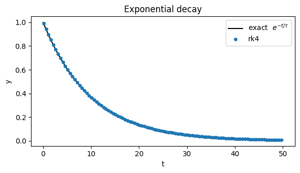
max abs error (rk4): 2.1823778006968553e-07

The Runge-Kutta solution sits right on top of the analytic curve — the error is at the level of floating-point noise for this smooth, well-conditioned problem.

Worked example 2 — a two-state system

A module can own several DiffEqStates. Here is an undamped harmonic oscillator,

\[\frac{dx}{dt} = v, \qquad \frac{dv}{dt} = -\omega^2 x,\]

which traces \(x(t) = \cos(\omega t)\) for \(x(0)=1,\ v(0)=0\). Each variable is its own DiffEqState, and compute_derivative fills both in one pass.

class Oscillator(brainstate.nn.Dynamics, DiffEqModule):
    def __init__(self, omega=1.0):
        super().__init__(in_size=1)
        self.omega = omega

    def init_state(self, *args):
        self.x = DiffEqState(jnp.ones(1))   # position, x(0) = 1
        self.v = DiffEqState(jnp.zeros(1))  # velocity, v(0) = 0

    def compute_derivative(self, *args):
        self.x.derivative = self.v.value
        self.v.derivative = -(self.omega ** 2) * self.x.value


osc = Oscillator(omega=2.0)
brainstate.nn.init_all_states(osc)
step = braincell.quad.get_integrator("rk4")

dt, n = 0.01, 1000
ts, xs = [], []
with brainstate.environ.context(dt=dt):
    for i in range(n):
        with brainstate.environ.context(t=i * dt):
            step(osc)
        ts.append((i + 1) * dt)
        xs.append(float(osc.x.value[0]))
ts, xs = np.array(ts), np.array(xs)

plt.figure(figsize=(6, 3.5))
plt.plot(ts, np.cos(2.0 * ts), "k-", label=r"exact  $\cos(\omega t)$")
plt.plot(ts[::40], xs[::40], "o", ms=4, label="rk4")
plt.xlabel("t"); plt.ylabel("x"); plt.legend(); plt.title("Harmonic oscillator")
plt.tight_layout(); plt.show()

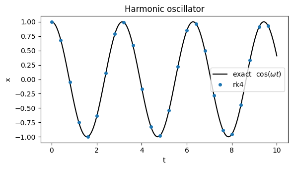
Both DiffEqStates are advanced together by the same solver step — you never integrate them by hand. That is the payoff of the protocol: you write the right-hand side, and braincell.quad does the stepping.

Where to go next

• Choosing and Using Solvers — the full solver catalog, how to pick one for stiff neural dynamics, and the high-level solver= shortcut.

• Advanced Integration — per-subsystem solvers, the stochastic diffusion slot, and registering your own integrator.