Choosing and Using Solvers

braincell.quad ships a family of numerical integrators. This page shows how to discover them, the two ways to apply them, and — most importantly — how to choose one for the stiff dynamics that are typical of biophysical neurons.

import brainstate
import brainunit as u
import numpy as np
import jax.numpy as jnp
import matplotlib.pyplot as plt

import braincell
from braincell import DiffEqState, DiffEqModule

The solver catalog

Integrators are grouped into categories. We can read them straight out of the registry.

registry = braincell.quad.get_registry()

by_cat = {}
for name in registry.names():
    entry = registry.entry(name)
    by_cat.setdefault(entry.category, []).append(name)

for category, names in sorted(by_cat.items()):
    print(f"{category:>12} : {sorted(names)}")

    explicit : ['euler', 'heun2', 'heun3', 'midpoint', 'ralston2', 'ralston3', 'ralston4', 'rk2', 'rk3', 'rk4', 'ssprk3']
 exponential : ['exp_euler', 'exp_exp_euler', 'ind_exp_euler']
    implicit : ['backward_euler', 'cn_exp_euler', 'cn_rk4', 'implicit_euler', 'implicit_exp_euler', 'implicit_rk4', 'splitting']
   staggered : ['staggered']
     voltage : ['dhs_voltage']

The families, in rough order of how often you reach for them in neural modeling:

Category	Examples	Character
explicit	euler, midpoint, rk2/3/4, heun*, ralston*, ssprk3	Classical Runge-Kutta. Cheap per step, high order available, but only conditionally stable — small dt required for stiff systems.
exponential	exp_euler, ind_exp_euler, exp_exp_euler	Treat the fast linear part exactly. Stable at large dt for the stiff gating dynamics of Hodgkin-Huxley neurons. The workhorse for point neurons.
implicit	backward_euler, implicit_euler/rk4, cn_*, splitting	Solve an implicit equation each step. Strong stability for very stiff problems at the cost of per-step linear solves.
staggered, voltage	staggered, dhs_voltage	Specialised schemes for multi-compartment cable equations.

Two ways to apply a solver

1. High-level: solver= on a cell

For a full neuron model you simply name the solver at construction. braincell wires the lifecycle and stepping for you. Below is a minimal Hodgkin-Huxley point neuron (the same recipe used in the single-compartment examples).

class HH(braincell.SingleCompartment):
    def __init__(self, size, solver="exp_euler"):
        super().__init__(size, solver=solver)
        self.na = braincell.ion.SodiumFixed(size, E=50. * u.mV)
        self.na.add(INa=braincell.channel.Na_HH1952(size))
        self.k = braincell.ion.PotassiumFixed(size, E=-77. * u.mV)
        self.k.add(IK=braincell.channel.K_HH1952(size))
        self.IL = braincell.channel.IL(size, E=-54.387 * u.mV,
                                       g_max=0.03 * (u.mS / u.cm ** 2))


def simulate(solver, dt=0.1, t_end=100.):
    neuron = HH(1, solver=solver)
    neuron.init_state()

    def step(t):
        with brainstate.environ.context(t=t):
            neuron.update(10. * u.nA / u.cm ** 2)   # constant drive
        return neuron.V.value

    with brainstate.environ.context(dt=dt * u.ms):
        times = u.math.arange(0. * u.ms, t_end * u.ms, brainstate.environ.get_dt())
        vs = brainstate.transform.for_loop(step, times)
    return np.asarray(times.to_decimal(u.ms)), np.asarray(u.math.squeeze(vs).to_decimal(u.mV))


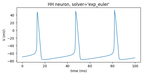
t, v = simulate("exp_euler")
plt.figure(figsize=(6, 3.2))
plt.plot(t, v, lw=1.2)
plt.xlabel("time (ms)"); plt.ylabel("V (mV)")
plt.title("HH neuron, solver='exp_euler'")
plt.tight_layout(); plt.show()

2. Low-level: call the step function directly

When you drive a bare DiffEqModule yourself (as in the previous page), fetch the step function from the registry and call it inside an environ context. This path works with the generic explicit Runge-Kutta solvers, which make no assumption about the model being a neuron.

class Decay(brainstate.nn.Dynamics, DiffEqModule):
    def __init__(self, tau=10.0):
        super().__init__(in_size=1)
        self.tau = tau

    def init_state(self, *args):
        self.y = DiffEqState(jnp.ones(1))

    def compute_derivative(self, *args):
        self.y.derivative = -self.y.value / self.tau


def run_decay(solver_name, dt=0.1, t_end=50.0):
    model = Decay(tau=10.0)
    brainstate.nn.init_all_states(model)
    step = braincell.quad.get_integrator(solver_name)
    n = int(t_end / dt)
    with brainstate.environ.context(dt=dt):
        for i in range(n):
            with brainstate.environ.context(t=i * dt):
                step(model)
            last_t = (i + 1) * dt
    return last_t, float(model.y.value[0])

run_decay("rk4")

(50.0, 0.006737955845892429)

Accuracy: order matters

On a smooth problem, a higher-order method reaches a given accuracy with far fewer, larger steps. Here is the global error at \(t=50\) for the decay problem (\(y(50) = e^{-5}\)) across three explicit schemes at the same dt.

exact = np.exp(-5.0)
print(f"{'solver':>10}  {'order':>5}  {'y(50)':>12}  {'abs error':>12}")
for name in ["euler", "midpoint", "rk4"]:
    order = braincell.quad.get_registry().entry(name).order
    _, y = run_decay(name, dt=0.5)
    print(f"{name:>10}  {order:>5}  {y:>12.3e}  {abs(y - exact):>12.3e}")

    solver  order         y(50)     abs error
     euler      1     5.921e-03     8.174e-04
  midpoint      2     6.753e-03     1.459e-05

       rk4      4     6.738e-03     9.306e-10

First-order Euler trails the fourth-order RK4 by several orders of magnitude at the same step size. For smooth problems, prefer a higher-order explicit method.

Stability: why neurons need special solvers

Accuracy is not the whole story. Hodgkin-Huxley gating variables relax on a sub-millisecond timescale while the spike itself plays out over milliseconds — the system is stiff. Explicit methods are only conditionally stable: push dt past a threshold and they blow up, no matter their order.

The demonstration below runs the same HH neuron at dt = 0.1 ms with an exponential integrator and with explicit RK4.

t_exp, v_exp = simulate("exp_euler", dt=0.1)
t_rk4, v_rk4 = simulate("rk4", dt=0.1)

print("exp_euler : max |V| =", f"{np.nanmax(np.abs(v_exp)):.1f} mV",
      "| any NaN:", bool(np.isnan(v_exp).any()))
print("rk4       : max |V| =", f"{np.nanmax(np.abs(v_rk4)):.1f} mV"
      if not np.isnan(v_rk4).all() else "nan",
      "| any NaN:", bool(np.isnan(v_rk4).any()))

plt.figure(figsize=(6, 3.2))
plt.plot(t_exp, v_exp, lw=1.2, label="exp_euler (stable)")
plt.xlabel("time (ms)"); plt.ylabel("V (mV)")
plt.title("Same neuron, same dt=0.1 ms")
plt.legend(); plt.tight_layout(); plt.show()

exp_euler : max |V| = 76.6 mV | any NaN: False
rk4       : max |V| = 158.2 mV | any NaN: True

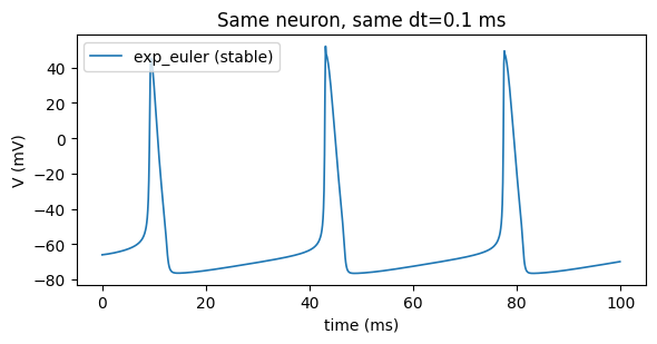
At dt = 0.1 ms exp_euler produces a clean spike train, while explicit RK4 diverges to NaN. This is why exponential integrators (exp_euler, ind_exp_euler) are the recommended choice for point neurons: they remain stable at the step sizes that make large simulations affordable. (The SingleCompartment default is the explicit rk2, so for stiff models you will usually want to pass solver=... explicitly.)

For a side-by-side comparison of several integrators on a neuron — including how the spike timing shifts between methods — see the worked example Effects of Different Integration Methods on HH Neuron Dynamics.

Choosing a solver — rules of thumb

• Point neurons (single compartment): start with exp_euler or ind_exp_euler. They are stable at dt = 0.1 ms and accurate enough for spike-level fidelity.

• Very stiff or near-equilibrium dynamics: an implicit method (backward_euler, implicit_exp_euler) trades per-step cost for robustness.

• Smooth, non-stiff sub-systems you drive yourself: the explicit Runge-Kutta family (rk4, midpoint) is simplest and works on any DiffEqModule.

• Multi-compartment cables: see the staggered / dhs_voltage schemes, which exploit the tree structure of the morphology.

The next page covers mixing solvers across sub-systems, the stochastic diffusion slot, and registering your own integrator.