
Cell in BrainCell#
This notebook is the direct sequel to 1.morphology.ipynb.
In the previous tutorial, we focused on geometry and topology. Here we move one layer upward and ask a new question:
How does a morphology become a simulation-ready cell object?
We will focus on four ideas:
Build a
Celldirectly from an existing morphology.Inspect control volumes (
CVs), which are the basic structural units of the cell layer.Compare different
cv_policychoices.Use the declarative APIs
paint(...)andplace(...).
To keep this notebook focused on the cell layer, we will load a ready-made morphology from ../../data/morphology/example_tree.swc instead of rebuilding one by hand.
import os

os.environ.setdefault("JAX_PLATFORMS", "cpu")

import braincell
import brainstate
import brainunit as u
import matplotlib.pyplot as plt

from braincell import Cell, Morphology
from braincell import CVPerBranch, MaxCVLen
from braincell.filter import BranchSlice, RootLocation, at
from braincell.mech import CableProperty, Channel, CurrentClamp, StateProbe
ERROR:2026-04-25 19:08:31,720:jax._src.xla_bridge:444: Jax plugin configuration error: Exception when calling jax_plugins.xla_cuda12.initialize()
Traceback (most recent call last):
  File "/home/swl/anaconda3/envs/braincell/lib/python3.10/site-packages/jax/_src/xla_bridge.py", line 442, in discover_pjrt_plugins
    plugin_module.initialize()
  File "/home/swl/anaconda3/envs/braincell/lib/python3.10/site-packages/jax_plugins/xla_cuda12/__init__.py", line 324, in initialize
    _check_cuda_versions(raise_on_first_error=True)
  File "/home/swl/anaconda3/envs/braincell/lib/python3.10/site-packages/jax_plugins/xla_cuda12/__init__.py", line 257, in _check_cuda_versions
    cublas_version = _version_check("cuBLAS", cuda_versions.cublas_get_version,
  File "/home/swl/anaconda3/envs/braincell/lib/python3.10/site-packages/jax_plugins/xla_cuda12/__init__.py", line 217, in _version_check
    raise RuntimeError(msg)
RuntimeError: Outdated cuBLAS installation found.
Version JAX was built against: 120803
Minimum supported: 120100
Installed version: 120001
The local installation version must be no lower than 120100.
# Keep any vis examples in this notebook aligned with the shared 2D/3D palette.
braincell.vis.configure_defaults(
    branch_type_colors={
        "soma": "#2f3136",
        "axon": "#6c8ead",
        "basal_dendrite": "#be866f",
        "apical_dendrite": "#d6ad62",
        "dendrite": "#9eaa84",
        "custom": "#9aa4af",
    },
)
VisDefaults(layout_2d_default='fan', shape_2d_default='frustum', mode_3d_default='geometry', branch_type_colors={'soma': (47, 49, 54), 'axon': (108, 142, 173), 'basal_dendrite': (190, 134, 111), 'apical_dendrite': (214, 173, 98), 'dendrite': (158, 170, 132), 'custom': (154, 164, 175)}, branch_type_edge_colors_2d=None, alpha_2d=0.8, alpha_2d_poly=None, alpha_2d_line=None, frustum_edge_linewidth_2d=0.9, alpha_3d_tube=1.0, highlight_color=(255, 215, 0), highlight_alpha=0.9, marker_color=(30, 144, 255), marker_size_2d=36.0, marker_radius_3d_um=1.5)
1. From morphology to Cell#
A Cell starts from a morphology, but it adds an important new layer: discretization.
Instead of working directly with whole branches, the cell layer works with control volumes (CVs). These are the structural units on which cable properties and mechanisms are assigned.
The simplest entry point is therefore:
load a morphology
pass it into
Cell(...)inspect the resulting CV structure
morpho = Morphology.from_swc("../../data/morphology/example_tree.swc")

print(morpho.topo())

cell = Cell(morpho)
print(cell)
soma
├── axon_0
│   └── axon_1
└── basal_dendrite_0
    ├── basal_dendrite_1
    │   ├── basal_dendrite_2
    │   └── basal_dendrite_3
    ├── basal_dendrite_4
    └── basal_dendrite_5
Cell(root='soma', n_branches=9, n_paint_rules=1, n_place_rules=0, initialized=False)
Useful Cell summary fields#
The compact string form of Cell shows a few high-level counters.
Field |
Meaning |
|---|---|
|
Name of the root branch in the cloned morphology |
|
Total number of morphology branches inside the cell |
|
Number of recorded |
|
Number of recorded |
The preview count cell.n_cv (and the full CV tuple cell.cvs) is computed lazily from the policy and paint rules — it is not part of the repr but is always available as a property.
print("n_cv:", cell.n_cv)
print("len(cell.cvs):", len(cell.cvs))
print("first three CV intervals:")
for cv in cell.cvs[:3]:
    print(f"  CV {cv.id}: branch_id={cv.branch_id}, branch_type={cv.branch_type}, prox={cv.prox}, dist={cv.dist}")
n_cv: 9
len(cell.cvs): 9
first three CV intervals:
  CV 0: branch_id=0, branch_type=soma, prox=0.0, dist=1.0
  CV 1: branch_id=1, branch_type=axon, prox=0.0, dist=1.0
  CV 2: branch_id=2, branch_type=axon, prox=0.0, dist=1.0
2. What is a CV?#
A CV (control volume) is the basic structural object in the cell layer.
Conceptually, one CV corresponds to one interval on one branch. It stores:
geometry, such as length and area
cable properties, such as
cm,ra,v, andtemptopology, such as parent/child CV relationships
attached mechanisms, split into
density_mechandpoint_mech
In other words, morphology tells us where the cable is, while CVs tell us where the cell model will actually live.
Useful CV attributes#
Attribute |
Meaning |
|---|---|
|
Unique CV index within the cell |
|
Which morphology branch this CV belongs to |
|
The branch type, such as |
|
Proximal boundary of the CV on its branch, in normalized branch coordinates |
|
Distal boundary of the CV on its branch, in normalized branch coordinates |
|
Parent CV id, or |
|
Child CV ids attached downstream |
|
Physical length of this CV |
|
Membrane area of this CV |
|
Membrane capacitance density at the CV midpoint |
|
Axial resistivity at the CV midpoint |
|
Resting / initial membrane potential at the CV midpoint |
|
Temperature stored at the CV midpoint |
|
Total axial resistance across the CV |
|
Axial resistance from the midpoint to the proximal end |
|
Axial resistance from the midpoint to the distal end |
|
Density mechanisms assigned to this CV |
|
Point mechanisms assigned to this CV |
cv0 = cell.cvs[0]
print(cv0)

# Identity and topology.
print("id:", cv0.id)
print("branch_id:", cv0.branch_id)
print("branch_type:", cv0.branch_type)
print("parent_cv:", cv0.parent_cv)
print("children_cv:", cv0.children_cv)

# Geometry.
print("length:", cv0.length)
print("area:", cv0.area)
print("r_axial:", cv0.r_axial)

# Cable properties defined at the CV midpoint.
print("cm:", cv0.cm)
print("ra:", cv0.ra)
print("v:", cv0.v)
print("temp:", cv0.temp)

# Mechanism containers are empty at this stage.
print("density_mech:", cv0.density_mech)
print("point_mech:", cv0.point_mech)
CV(id=0, branch_id=0, branch_type='soma', prox=0.0, dist=1.0, parent_cv=None, children_cv=(1, 3), length=Quantity(10., "um"), area=Quantity(314.15927, "um^2"), cm=Quantity(1., "uF / cm^2"), ra=Quantity(100., "cm * ohm"), v=Quantity(-65., "mV"), temp=Quantity(309.15, "K"), r_axial=Quantity(127323.95, "ohm"), r_axial_prox=Quantity(63661.977, "ohm"), r_axial_dist=Quantity(63661.977, "ohm"), radius_prox=Quantity(5., "um"), radius_mid=Quantity(5., "um"), radius_dist=Quantity(5., "um"), density_mech=(), point_mech=())
id: 0
branch_id: 0
branch_type: soma
parent_cv: None
children_cv: (1, 3)
length: 10. um
area: 314.15927 um^2
r_axial: 127323.95 ohm
cm: 1. uF / cm^2
ra: 100. cm * ohm
v: -65. mV
temp: 309.15 K
density_mech: ()
point_mech: ()
3. CV policies#
The morphology does not uniquely determine the number of CVs. That job belongs to the CV policy.
Three useful cases are:
Cell(morpho): use the defaultCVPerBranch()policyCell(morpho, cv_policy=CVPerBranch(cv_per_branch=2)): force every branch to use two CVsCell(morpho, cv_policy=MaxCVLen(max_cv_len=...)): choose the number of CVs automatically from physical branch length
This is the main structural knob of the cell layer.
default_cell = Cell(morpho)
split_cell = Cell(morpho, cv_policy=CVPerBranch(cv_per_branch=2))
auto_cell = Cell(morpho, cv_policy=MaxCVLen(max_cv_len=20.0 * u.um))

print("default policy")
print(default_cell)
print()
print("CVPerBranch(cv_per_branch=2)")
print(split_cell)
print()
print("MaxCVLen(max_cv_len=20 um)")
print(auto_cell)
print()
print("first four CV intervals under CVPerBranch(cv_per_branch=2):")
for cv in split_cell.cvs[:4]:
    print(f"  CV {cv.id}: branch_id={cv.branch_id}, prox={cv.prox}, dist={cv.dist}")
default policy
Cell(root='soma', n_branches=9, n_paint_rules=1, n_place_rules=0, initialized=False)

CVPerBranch(cv_per_branch=2)
Cell(root='soma', n_branches=9, n_paint_rules=1, n_place_rules=0, initialized=False)

MaxCVLen(max_cv_len=20 um)
Cell(root='soma', n_branches=9, n_paint_rules=1, n_place_rules=0, initialized=False)

first four CV intervals under CVPerBranch(cv_per_branch=2):
  CV 0: branch_id=0, prox=0.0, dist=0.5
  CV 1: branch_id=0, prox=0.5, dist=1.0
  CV 2: branch_id=1, prox=0.0, dist=0.5
  CV 3: branch_id=1, prox=0.5, dist=1.0
4. The node tree#
A Cell holds only declarations. The execution-oriented view — the node tree — is built later, together with all runtime state, by calling cell.init_state(), which flips the cell into its INITIALIZED phase.
For this tutorial you only need two facts:
cell.cvsis the membrane-oriented view, available directly on the declarationcell.node_treeis the point/edge execution view, available aftercell.init_state()runs
split_cell.init_state()
node_tree = split_cell.node_tree
print(node_tree)
print("n_nodes:", len(node_tree.nodes))
print("n_edges:", len(node_tree.edges))
print("expected n_nodes = n_cv + n_branches + 1:", split_cell.n_cv + len(split_cell.morpho.branches) + 1)
-----------------------------------
n_nodes       | 28
n_edges        | 27
root_node_id  | 0
-----------------------------------

n_nodes: 28
n_edges: 27
expected n_nodes = n_cv + n_branches + 1: 28
5. paint(...): declarative region-based assignment#
paint(...) is the main API for assigning properties or density mechanisms over a region of the cell.
Its general shape is:
cell.paint(region, *mechanisms)
Here:
regionis a region expression such asBranchSlice(...)the remaining arguments are declarative mechanism objects
A useful mental model is that paint(...) does not directly run a mechanism. It declares what should exist on which part of the cell.
Painting cable properties#
Every Cell starts with one default global cable-property rule. A later paint(...) call can locally override those midpoint properties on the CVs that fall inside the painted region.
cable_cell = Cell(morpho, cv_policy=CVPerBranch(cv_per_branch=2))
cable_cell.paint(
    BranchSlice(branch_index=0, prox=0.0, dist=1.0),
    CableProperty(
        resting_potential=-70.0 * u.mV,
        membrane_capacitance=2.0 * (u.uF / u.cm ** 2),
        axial_resistivity=200.0 * (u.ohm * u.cm),
        temperature=u.celsius2kelvin(20.0),
    ),
)

print(cable_cell)
print("painted soma CV example:")
print("v:", cable_cell.cvs[0].v)
print("cm:", cable_cell.cvs[0].cm)
print("ra:", cable_cell.cvs[0].ra)
print("temp:", cable_cell.cvs[0].temp)
Cell(root='soma', n_branches=9, n_paint_rules=2, n_place_rules=0, initialized=False)
painted soma CV example:
v: -70. mV
cm: 2. uF / cm^2
ra: 200. cm * ohm
temp: 293.15 K
Painting a density mechanism#
A density mechanism is distributed over a region rather than attached to a single point.
In the example below, Channel("IL", ...) is a declarative channel specification. The cell runtime lowers it into a dense layout over the active CV midpoints.
channel_cell = Cell(morpho)
channel_cell.paint(
    BranchSlice(branch_index=[0, 1], prox=0.0, dist=1.0),
    Channel("IL", g_max=4.0 * (u.mS / u.cm ** 2), E=-68.0 * u.mV),
)

# All runtime inspection — layouts, per-point state — lives on the Cell after init_state().
channel_cell.init_state()
layout = channel_cell.layouts[0]
point_id = int(layout.point_index[0])

print("layout.kind:", layout.kind)
print("layout.target:", layout.target)
print("layout.n_active:", layout.n_active)
print("layout.source_cv_ids:", layout.source_cv_ids)
print("layout.point_index:", layout.point_index.tolist())
print("sample g_max at one active point:", channel_cell.get_point_state(point_id)[layout.id]["g_max"])
print("sample E at one active point:", channel_cell.get_point_state(point_id)[layout.id]["E"])
layout.kind: channel:IL
layout.target: density
layout.n_active: 2
layout.source_cv_ids: (0, 1)
layout.point_index: [1, 3]
sample g_max at one active point: 4. mS / cm^2
sample E at one active point: -68. mV
6. place(...): declarative point mechanisms#
place(...) is the companion API for mechanisms that should live at a single location instead of over a region.
Its general shape is:
cell.place(locset, *mechanisms)
Here:
locsetis a location expression such asRootLocation(...)the remaining arguments are point mechanisms such as
CurrentClamp
This is the right API for clamps, probes, and other point-like declarations.
place_cell = Cell(morpho, cv_policy=CVPerBranch(2))
place_cell.place(
    RootLocation(x=0.5),
    CurrentClamp(delay=1.0 * u.ms, durations=2.0 * u.ms, amplitudes=0.1 * u.nA),
)

place_cell.init_state()
layout = place_cell.layouts[0]

print(place_cell)
print("layout.kind:", layout.kind)
print("layout.target:", layout.target)
print("layout.n_active:", layout.n_active)
print("layout.point_index:", layout.point_index.tolist())
print("amplitudes:", place_cell.get_state(layout.id, "amplitudes"))
print("durations:", place_cell.get_state(layout.id, "durations"))
print("start:", place_cell.get_state(layout.id, "start"))
Cell(root='soma', n_cv=18, n_point=28, initialized=True)
layout.kind: CurrentClamp
layout.target: point
layout.n_active: 1
layout.point_index: [2]
amplitudes: [[0.1]] nA
durations: [[2.]] ms
delay: [1.] ms
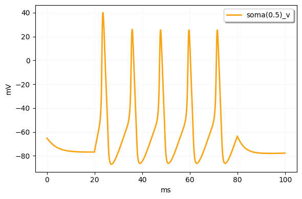
7. A minimal simulation#
So far we have only declared structure and mechanisms. To actually run the cell, we follow a two-step recipe:
Call
cell.init_state()to lower the declaration and allocate runtime state on the sameCell.Call
cell.run(dt=..., duration=...)to advance it over time. (runauto-callsinit_state()on first use.)
Cell has two phases: DECLARING (paint/place/config mutable) and INITIALIZED (runtime surface live). reset() returns a cell to DECLARING while keeping paint/place rules so you can re-initialize.
We use a simple HH-style configuration:
passive leak current
ILsodium current
Nav1p6_MA24_PCpotassium current
IK_HH1952a point current clamp at the root midpoint
a
StateProbeon the soma recording membrane voltage
sim_cell = Cell(
    morpho,
    cv_policy=CVPerBranch(cv_per_branch=2),
    solver="staggered",
)

sim_cell.paint(
    BranchSlice(branch_index=[0, 1], prox=0.0, dist=1.0),
    Channel("IL", g_max=0.03 * (u.mS / u.cm ** 2), E=-54.387 * u.mV),
    Channel("Na_HH1952", g_max=120.0 * (u.mS / u.cm ** 2)),
    Channel("K_HH1952", g_max=36.0 * (u.mS / u.cm ** 2)),
)

sim_cell.place(
    RootLocation(x=0.5),
    CurrentClamp(delay=20.0 * u.ms, durations=60.0 * u.ms, amplitudes=0.2 * u.nA),
)

sim_cell.place(
    at("soma", 0.5),
    StateProbe(),
)

sim_cell.init_state()
sim_cell.reset_state()
# init_state() already called above

dt = 0.1 * u.ms
duration = 100.0 * u.ms

result1 = sim_cell.run(dt=dt, duration=duration)

times_ms = u.math.concatenate([result1.time])
vs_mV = u.math.concatenate([
    result1.traces["soma(0.5)_v"],
])


plt.rcParams['font.family'] = 'DejaVu Sans'
plt.style.use('default')
fig, ax = plt.subplots(figsize=(6, 4))
line, = ax.plot(times_ms, vs_mV, label="soma(0.5)_v", linewidth=2, color="#f8a413")
ax.fill_between(times_ms, vs_mV, alpha=0., color="#ffffff")
# ax.set_xlabel("Time (ms)", fontsize=14)
# ax.set_ylabel("Voltage (mV)", fontsize=14)
ax.legend(frameon=True, fancybox=True, shadow=True, loc='best')
ax.grid(True, linestyle='-', alpha=0.15, linewidth=0.5)
plt.tight_layout()
plt.show()


# fig, axes = plt.subplots(1, 1, figsize=(5, 5))
# sim_cell.vis_cv(
#     value="V",
#     cmap="viridis",
#     vmin=-80.0,
#     vmax=-40.0,
#     value_label="Voltage",
#     ax=axes,  # note: with subplots(1, 1), axes is a single object, not a list
#     show=False,
# )
# plt.show()  # add this line to render
Summary#
You have now seen the main ideas of the cell layer in BrainCell:
A
Cellstarts in DECLARING — morphology, CV policy,paint(...)rules,place(...)rules are freely mutable.init_state()transitions it to INITIALIZED, where the runtime surface is live.Discretization produces a list of
CVs; the CV policy is the main structural knob.cell.init_state()lowers the declaration and allocates the runtime (node tree, layouts, integrator state, probes) on the sameCell.All runtime inspection (
layouts,get_point_state(...),get_state(...),node_tree,run(...),current_time,sample_probes()) is available on theCellafterinit_state()(and raisesRuntimeErrorin DECLARING).Building twice produces two independent runnables, so a single declaration can seed many parallel simulations.
A natural next step is 3.vis.ipynb, where the structural and runtime views become easier to inspect visually.