Single-cell Frontend: Morphology, Visualization, and Model Decoration

This notebook is a concise stage summary of BrainCell’s single-cell frontend. It covers morphology ingestion, geometry and topology views, declarative regions and locations, mechanism placement, and the current interaction boundary. It deliberately does not run a simulation or discuss numerical performance and networks.

Area	Available now	Design reference	Next step
Ingestion	SWC and Neurolucida ASC readers with structured reports	Common reconstruction formats	Interactive validation and repair
Morphology views	2D projection, tree layouts, 3D geometry and skeleton views	Morphology viewers and publication workflows	Persistent selection and editing
Model topology	Branch, control-volume, and runtime-node views	Multi-compartment model structure	Synchronized inspection across levels
Model decoration	Region/locset expressions plus paint and place	Arbor labels and decorations	Visual region, channel, and synapse editors
Interaction	Backend-independent pick, hover, and leave callbacks	Interactive scientific visualization	Undoable edits and Python export

For deeper coverage, see the morphology tutorial, filter tutorial, mechanism tutorial, and visualization tutorial.

Setup

The examples use repository fixtures and execute on CPU for reproducibility. Static figures are kept in docs/_static/single_cell_frontend/ so they can also be reused in reports and presentations.

from pathlib import Path
from contextlib import redirect_stderr
from io import StringIO
import logging
import os
import warnings

os.environ.setdefault("JAX_PLATFORMS", "cpu")
os.environ.setdefault("MPLBACKEND", "Agg")
os.environ.setdefault("PYVISTA_OFF_SCREEN", "true")

import brainunit as u
import matplotlib.pyplot as plt
from IPython.display import Image, display

import braincell.mech as mech
import braincell.vis as vis
from braincell import Cell, MaxCVLen, Morphology
from braincell.filter import AllRegion, RootLocation, Terminals, branch_in, branch_range

DATA = Path("../../data/morphology")
OUTPUT = Path("../_static/single_cell_frontend")
OUTPUT.mkdir(parents=True, exist_ok=True)

plt.rcParams.update({
    "figure.facecolor": "white",
    "axes.facecolor": "white",
    "axes.spines.top": False,
    "axes.spines.right": False,
    "font.size": 10,
})
logging.getLogger("matplotlib").setLevel(logging.ERROR)

def save_figure(fig, name):
    path = OUTPUT / name
    fig.savefig(path, dpi=200, bbox_inches="tight", facecolor="white")
    return path

import braincell.vis as vis

vis.configure_defaults(
    branch_type_colors={
        "soma": "#090909",
        "axon": "#0076D7",
        "dendrite": "#D42607",
        "basal_dendrite": "#FD4C0B",
        "apical_dendrite": "#FF1111",
        "custom": "#006D3E",
    },
    highlight_color="#9504D9",
    marker_color="#1E90FF",
)

VisDefaults(layout_2d_default='fan', shape_2d_default='frustum', mode_3d_default='geometry', branch_type_colors={'soma': (9, 9, 9), 'axon': (0, 118, 215), 'basal_dendrite': (253, 76, 11), 'apical_dendrite': (255, 17, 17), 'dendrite': (212, 38, 7), 'custom': (0, 109, 62)}, branch_type_edge_colors_2d=None, alpha_2d=0.8, alpha_2d_poly=None, alpha_2d_line=None, frustum_edge_linewidth_2d=0.9, alpha_3d_tube=1.0, highlight_color=(149, 4, 217), highlight_alpha=0.9, marker_color=(30, 144, 255), marker_size_2d=36.0, marker_radius_3d_um=1.5)

Part 1 — Morphology ingestion

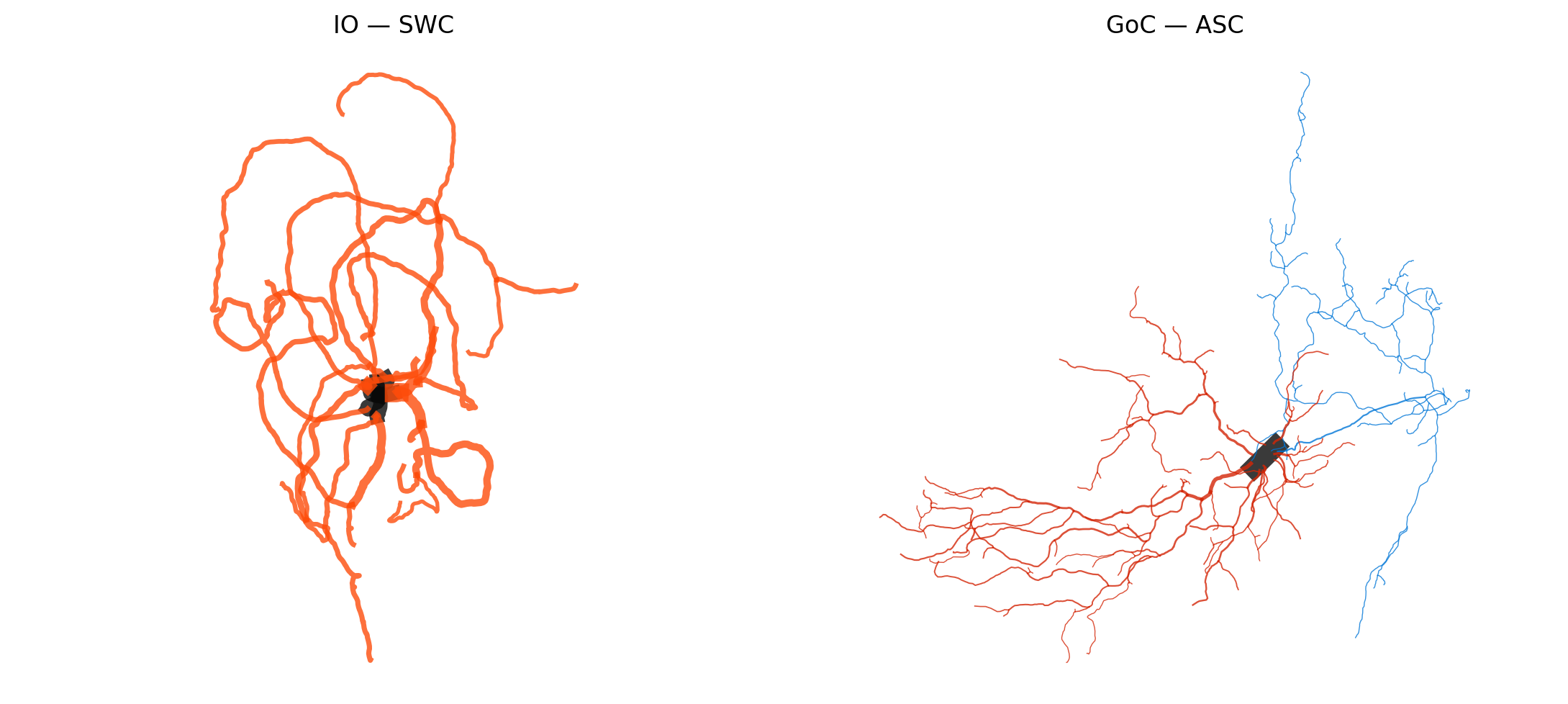
Morphology.from_swc and Morphology.from_asc normalize different reconstruction formats into the same tree model. The optional reports keep validation information beside the imported morphology. Here, an inferior olivary cell exercises the SWC path and a Golgi cell exercises the ASC path.

with warnings.catch_warnings(), redirect_stderr(StringIO()):
    warnings.filterwarnings("ignore", message="from_points produced.*")
    io, io_report = Morphology.from_swc(DATA / "io.swc", return_report=True)
    goc, goc_report = Morphology.from_asc(DATA / "goc.asc", return_report=True)

print(f"IO / SWC reader report:  {io_report.error_count} errors, {io_report.warning_count} warnings")
print(io.metric)
print(f"GoC / ASC reader report: {goc_report.error_count} errors, {goc_report.warning_count} warnings")
print(goc.metric)

Warning: no DISPLAY environment variable.
--No graphics will be displayed.

IO / SWC reader report:  0 errors, 2 warnings
-----------------------------------
n_branches       | 31
n_stems          | 6
n_bifurcations   | 11
max_branch_order | 5
total_length     | 2601.70 um
mean_radius      | 1.41 um
total_area       | 23278.34 um^2
total_volume     | 19109.84 um^3
max_path_dist    | 303.73 um
-----------------------------------

GoC / ASC reader report: 0 errors, 0 warnings
-----------------------------------
n_branches       | 227
n_stems          | 12
n_bifurcations   | 108
max_branch_order | 13
total_length     | 4985.44 um
mean_radius      | 0.31 um
total_area       | 9806.74 um^2
total_volume     | 3252.68 um^3
max_path_dist    | 513.82 um
-----------------------------------

fig, axes = plt.subplots(1, 2, figsize=(11, 5))
for ax, morpho, title in zip(axes, (io, goc), ("IO — SWC", "GoC — ASC")):
    vis.plot2d(morpho, layout="projected", shape="line", ax=ax)
    ax.set_title(title)
fig.tight_layout()
ingestion_path = save_figure(fig, "ingestion_comparison.png")
plt.close(fig)
display(Image(filename=ingestion_path))

Part 2 — 2D and 3D morphology views

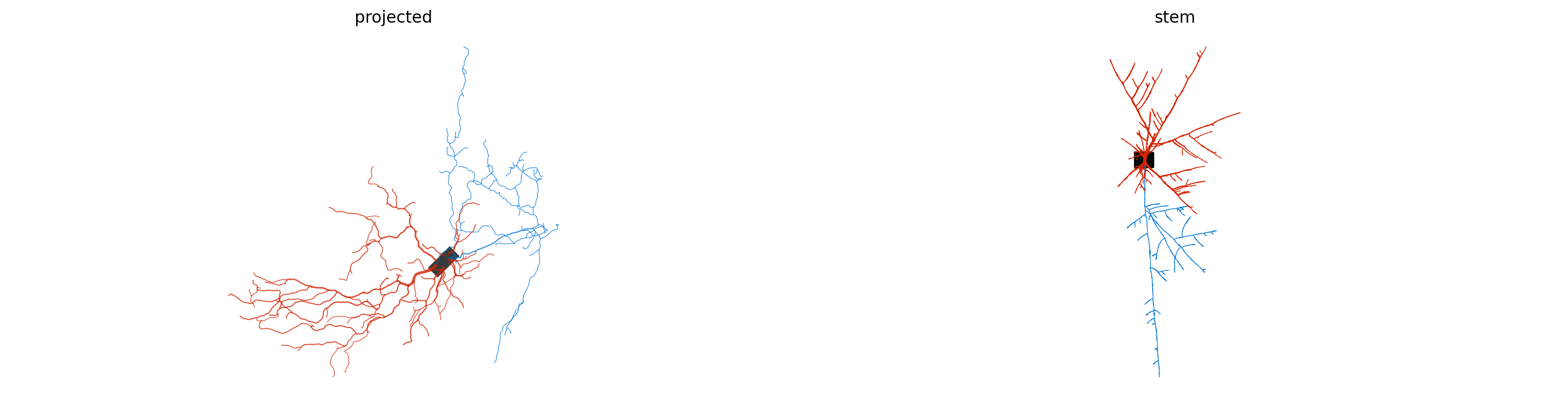
The 2D API separates the underlying morphology from its presentation. projected preserves a physical coordinate plane, while stem, balloon, and radial_360 expose tree structure with different layout strategies. The same morphology can also be rendered as full 3D geometry or as a lightweight skeleton.

layouts = ("projected", "stem") # , "balloon", "radial_360"
fig, axes = plt.subplots(1, 2, figsize=(16, 4.2))

for ax, layout in zip(axes, layouts):
    vis.plot2d(goc, layout=layout, shape="line", ax=ax)
    ax.set_title(layout)

fig.tight_layout()
layout_path = save_figure(fig, "layout_gallery.png")
plt.close(fig)
display(Image(filename=layout_path))

# The static capture was rendered out-of-process with:
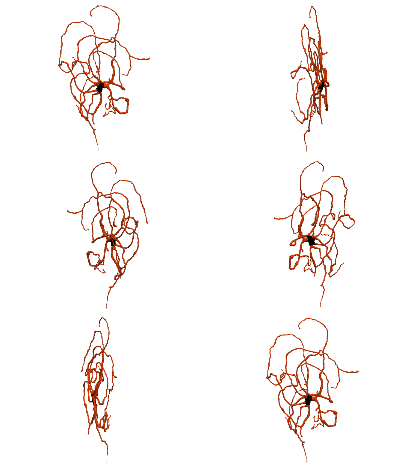
vis.plot3d(io, mode="geometry", backend="pyvista", jupyter_backend='html')

High-resolution rotating 3D captures

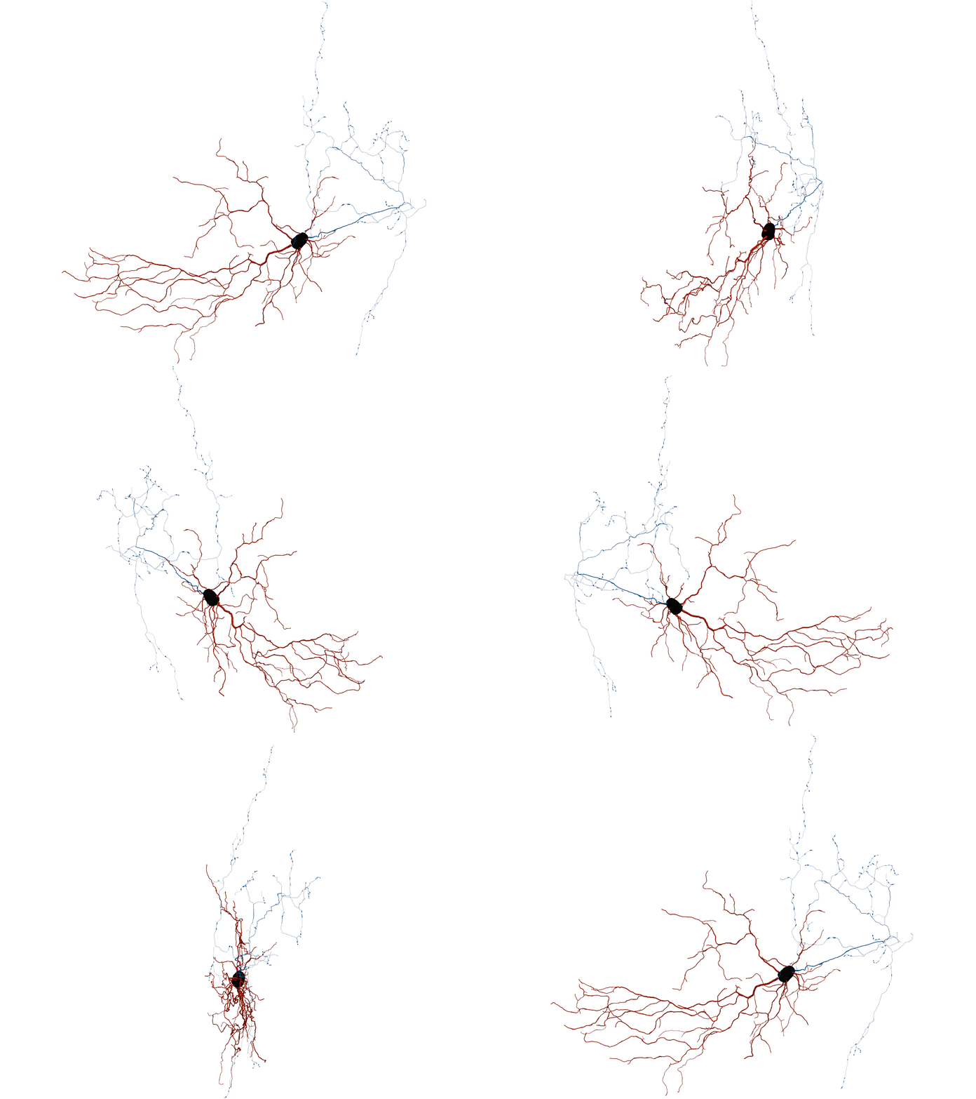
The interactive view above is retained for inspection. The helper below renders a presentation-ready GIF by orbiting the camera around the morphology’s vertical (Y) axis. Parallel projection and a fixed fit keep the apparent scale stable as the view moves from front to side to back. With parallel projection, zoom controls the apparent size while camera_distance_factor mainly controls camera and clipping distance.

import numpy as np
from PIL import Image as PILImage
from IPython.utils.capture import capture_output


def save_rotating_morphology_gif(
    morpho,
    filename,
    *,
    window_size=(1280, 960),
    n_frames=120,
    fps=30,
    start_angle_deg=90.0,
    rotation_deg=360.0,
    elevation_deg=8.0,
    camera_distance_factor=3.0,
    zoom=1.0,
    fit_margin=1.06,
    mode="geometry",
):
    """Render a smooth, upright Y-axis orbit as an animated GIF."""
    if n_frames < 2 or not 0 < fps <= 100:
        raise ValueError("n_frames must be >= 2 and fps must be in (0, 100].")
    if not -89 < elevation_deg < 89:
        raise ValueError("elevation_deg must be between -89 and 89.")
    if camera_distance_factor <= 0 or zoom <= 0 or fit_margin <= 0:
        raise ValueError("Camera distance, zoom, and fit margin must be positive.")

    output_path = OUTPUT / filename
    plotter = None
    try:
        with capture_output(), redirect_stderr(StringIO()):
            plotter = vis.plot3d(
                morpho, mode=mode, backend="pyvista", notebook=False
            )
            plotter.set_background("white")
            plotter.hide_axes()
            plotter.window_size = window_size
            plotter.show(auto_close=False, interactive=False)

        bounds = np.array([
            [plotter.bounds.x_min, plotter.bounds.x_max],
            [plotter.bounds.y_min, plotter.bounds.y_max],
            [plotter.bounds.z_min, plotter.bounds.z_max],
        ], dtype=float)
        center = bounds.mean(axis=1)
        corners = np.array([
            [x, y, z]
            for x in bounds[0]
            for y in bounds[1]
            for z in bounds[2]
        ])
        radius = np.linalg.norm(bounds[:, 1] - bounds[:, 0]) / 2.0
        camera_distance = max(radius * camera_distance_factor, 1.0)
        aspect = window_size[0] / window_size[1]
        elevation = np.deg2rad(elevation_deg)
        angles = np.linspace(
            start_angle_deg,
            start_angle_deg + rotation_deg,
            n_frames,
            endpoint=False,
        )

        world_up = np.array([0.0, 1.0, 0.0])
        camera_poses = []
        required_scales = []
        for angle_deg in angles:
            angle = np.deg2rad(angle_deg)
            radial = np.array([
                np.cos(angle) * np.cos(elevation),
                np.sin(elevation),
                np.sin(angle) * np.cos(elevation),
            ])
            camera_position = center + camera_distance * radial
            forward = center - camera_position
            forward /= np.linalg.norm(forward)
            camera_up = world_up - np.dot(world_up, forward) * forward
            camera_up /= np.linalg.norm(camera_up)
            camera_right = np.cross(forward, camera_up)
            camera_right /= np.linalg.norm(camera_right)

            relative_corners = corners - center
            half_height = np.max(np.abs(relative_corners @ camera_up))
            half_width = np.max(np.abs(relative_corners @ camera_right))
            required_scales.append(max(half_height, half_width / aspect))
            camera_poses.append((camera_position, camera_up))

        parallel_scale = max(required_scales) * fit_margin / zoom
        frames = []
        for camera_position, camera_up in camera_poses:
            plotter.camera_position = [
                tuple(camera_position), tuple(center), tuple(camera_up)
            ]
            plotter.camera.parallel_projection = True
            plotter.camera.parallel_scale = parallel_scale
            plotter.reset_camera_clipping_range()
            plotter.render()
            frame = plotter.screenshot(return_img=True)
            frames.append(PILImage.fromarray(frame).convert("RGB"))

        # GIF delays are stored in centiseconds; distribute rounding error
        # so the complete loop still has the requested average frame rate.
        frame_ends_cs = np.rint(np.arange(1, n_frames + 1) * 100 / fps).astype(int)
        frame_starts_cs = np.concatenate(([0], frame_ends_cs[:-1]))
        durations_ms = np.maximum(frame_ends_cs - frame_starts_cs, 1) * 10
        frames[0].save(
            output_path,
            save_all=True,
            append_images=frames[1:],
            duration=durations_ms.tolist(),
            loop=0,
            disposal=2,
            optimize=False,
        )
    finally:
        if plotter is not None:
            plotter.close()

    return output_path

# Presentation-quality defaults. Reduce size/frames/fps for a quicker draft.
GIF_WINDOW_SIZE = (1280, 960)
GIF_N_FRAMES = 120
GIF_FPS = 30
GIF_START_ANGLE_DEG = 90.0
GIF_ROTATION_DEG = 360.0
GIF_ELEVATION_DEG = 8.0
GIF_CAMERA_DISTANCE_FACTOR = 3.0
GIF_FIT_MARGIN = 1.06

common_gif_options = dict(
    window_size=GIF_WINDOW_SIZE,
    n_frames=GIF_N_FRAMES,
    fps=GIF_FPS,
    start_angle_deg=GIF_START_ANGLE_DEG,
    rotation_deg=GIF_ROTATION_DEG,
    elevation_deg=GIF_ELEVATION_DEG,
    camera_distance_factor=GIF_CAMERA_DISTANCE_FACTOR,
    fit_margin=GIF_FIT_MARGIN,
)
io_gif_path = save_rotating_morphology_gif(
    io, "io_3d_rotation.gif", zoom=1.08, **common_gif_options
)
goc_gif_path = save_rotating_morphology_gif(
    goc, "goc_3d_rotation.gif", zoom=1.20, **common_gif_options
)

print(f"IO rotating 3D:  {io_gif_path}")
display(Image(filename=io_gif_path, width=800))
print(f"GoC rotating 3D: {goc_gif_path}")
display(Image(filename=goc_gif_path, width=800))

IO rotating 3D:  ../_static/single_cell_frontend/io_3d_rotation.gif

GoC rotating 3D: ../_static/single_cell_frontend/goc_3d_rotation.gif

Part 3 — Branch, control-volume, and runtime-node topology

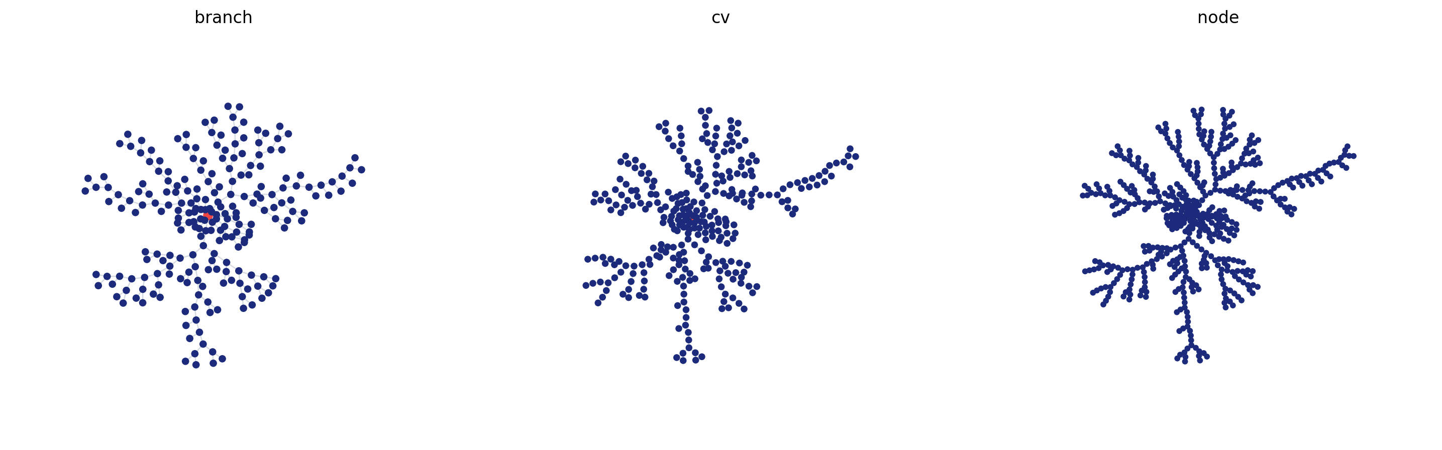
A single morphology supports several useful abstraction levels. Branch views emphasize biological tree structure; control-volume views show discretization; runtime-node views expose the graph consumed by mechanisms. The cell is initialized only to build these structures—no time stepping is performed.

soma = branch_in("type", "soma")
dendrites = branch_in("type", "dendrite")
thick = branch_range("mean_radius", (0.4 * u.um, None), closed="neither", )

sites = RootLocation(0.5) | Terminals()

cell = Cell(goc, cv_policy=MaxCVLen(40 * u.um))
cell.paint(
    AllRegion(),
    mech.Channel("IL", g_max=0.03 * u.mS / u.cm**2, E=-70 * u.mV),
)
cell.paint(
    dendrites,
    mech.Channel("Na_HH1952", g_max=120 * u.mS / u.cm**2),
)
cell.place(
    sites,
    mech.Synapse("ExpSyn", tau=2 * u.ms, e=0 * u.mV, weight=0.001 * u.uS),
)
cell.init_state()

print(f"branches: {cell.morpho.n_branches}")
print(f"control volumes: {cell.n_cv}")
print(f"runtime nodes: {len(cell.node_tree.nodes)}")
print(f"paint rules: {len(cell.paint_rules)}; place rules: {len(cell.place_rules)}")

branches: 227
control volumes: 309
runtime nodes: 537
paint rules: 3; place rules: 1

fig, axes = plt.subplots(1, 3, figsize=(15, 4.5))
for ax, level in zip(axes, ("branch", "cv", "node")):
    cell.vis_topology(
        level=level,
        region=soma,
        layout="kamada_kawai",
        ax=ax,
        show=False,
    )
    ax.set_title(level)

fig.tight_layout()
topology_path = save_figure(fig, "topology_levels.png")
plt.close(fig)
display(Image(filename=topology_path))

Part 4 — Regions, locations, and model decoration

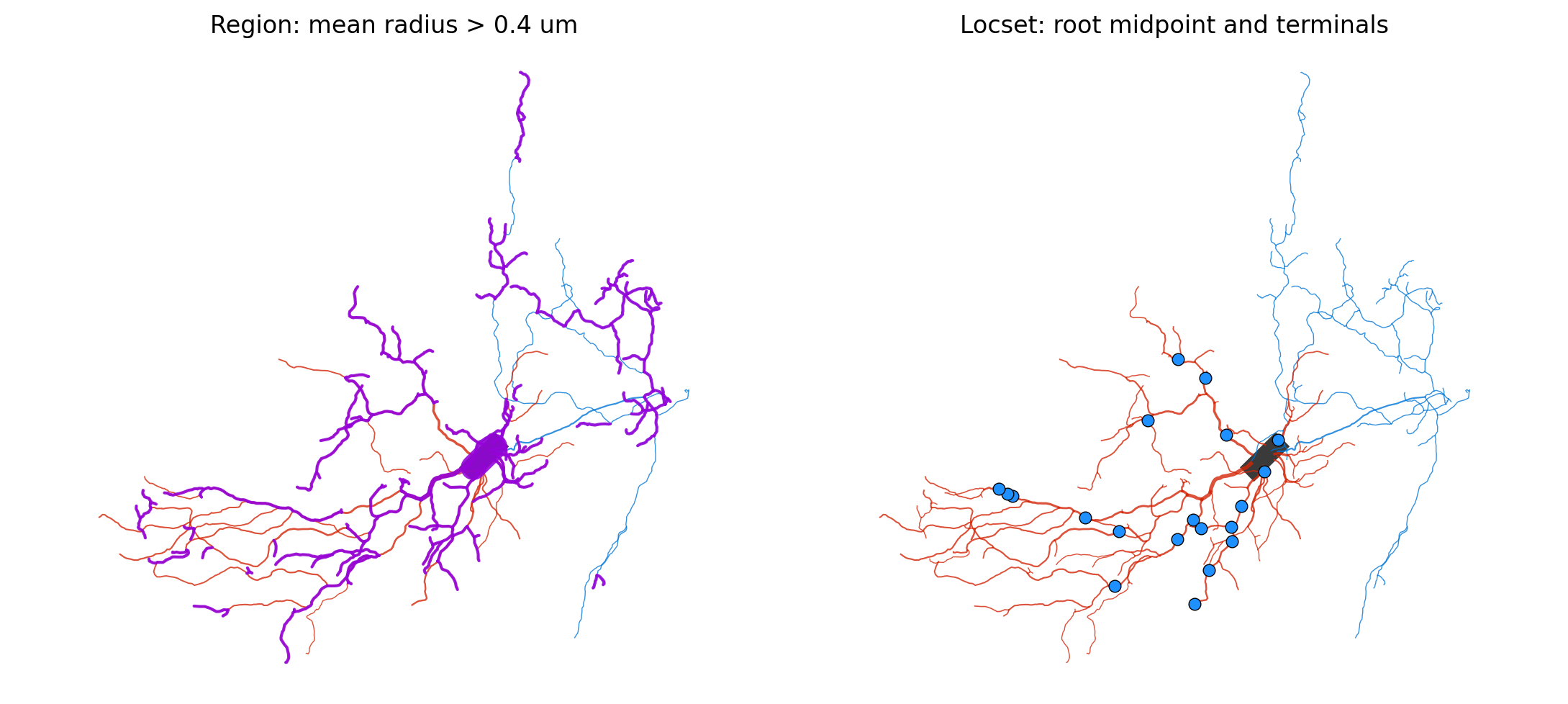
BrainCell follows the same separation of concerns used by Arbor’s regions and locsets: a region describes a continuous part of the cable tree, while a locset describes discrete sites. paint assigns distributed mechanisms to regions and place assigns point mechanisms to locations. The expressions stay reusable across visualization and model construction.

from braincell.filter import AllRegion, RandomSamples
dendrite_mask = goc.select(dendrites)


site_mask = goc.select(sites)

random_sampling = RandomSamples(
    region=thick,
    count=20,
    seed=42,
)
random_sampling_mask = goc.select(random_sampling)

long = branch_range("length", (None,40 * u.um,), closed="neither", )
thick_mask = goc.select(thick)

long_mask = goc.select(long)

fig, axes = plt.subplots(1, 2, figsize=(11, 5))
vis.plot2d(goc, layout="projected", shape="line", region=long_mask, ax=axes[0])
axes[0].set_title("Region: mean radius > 0.4 um")
vis.plot2d(goc, layout="projected", shape="line", locset=random_sampling_mask, ax=axes[1])
axes[1].set_title("Locset: root midpoint and terminals")


fig.tight_layout()
selection_path = save_figure(fig, "region_locset_overlays.png")
plt.close(fig)
display(Image(filename=selection_path))

Placing synapses on a locset

The same locset used for visualization can be passed directly to Cell.place. This example places one ExpSyn instance at the GoC root midpoint and at every terminal location.

synapse_cell = Cell(goc, cv_policy=MaxCVLen(40 * u.um))
synapse_cell.place(
    sites,
    mech.Synapse(
        "ExpSyn",
        name="selected_exp_syn",
        tau=2 * u.ms,
        e=0 * u.mV,
        weight=0.001 * u.uS,
    ),
)
synapse_cell.init_state()

synapse_layout = next(
    layout for layout in synapse_cell.layouts
    if layout.kind == "synapse:ExpSyn"
)
print(f"Selected locset locations: {len(site_mask.points)}")
print(f"Placed ExpSyn instances: {synapse_layout.n_active}")

Selected locset locations: 120
Placed ExpSyn instances: 120

Callable channel distributions

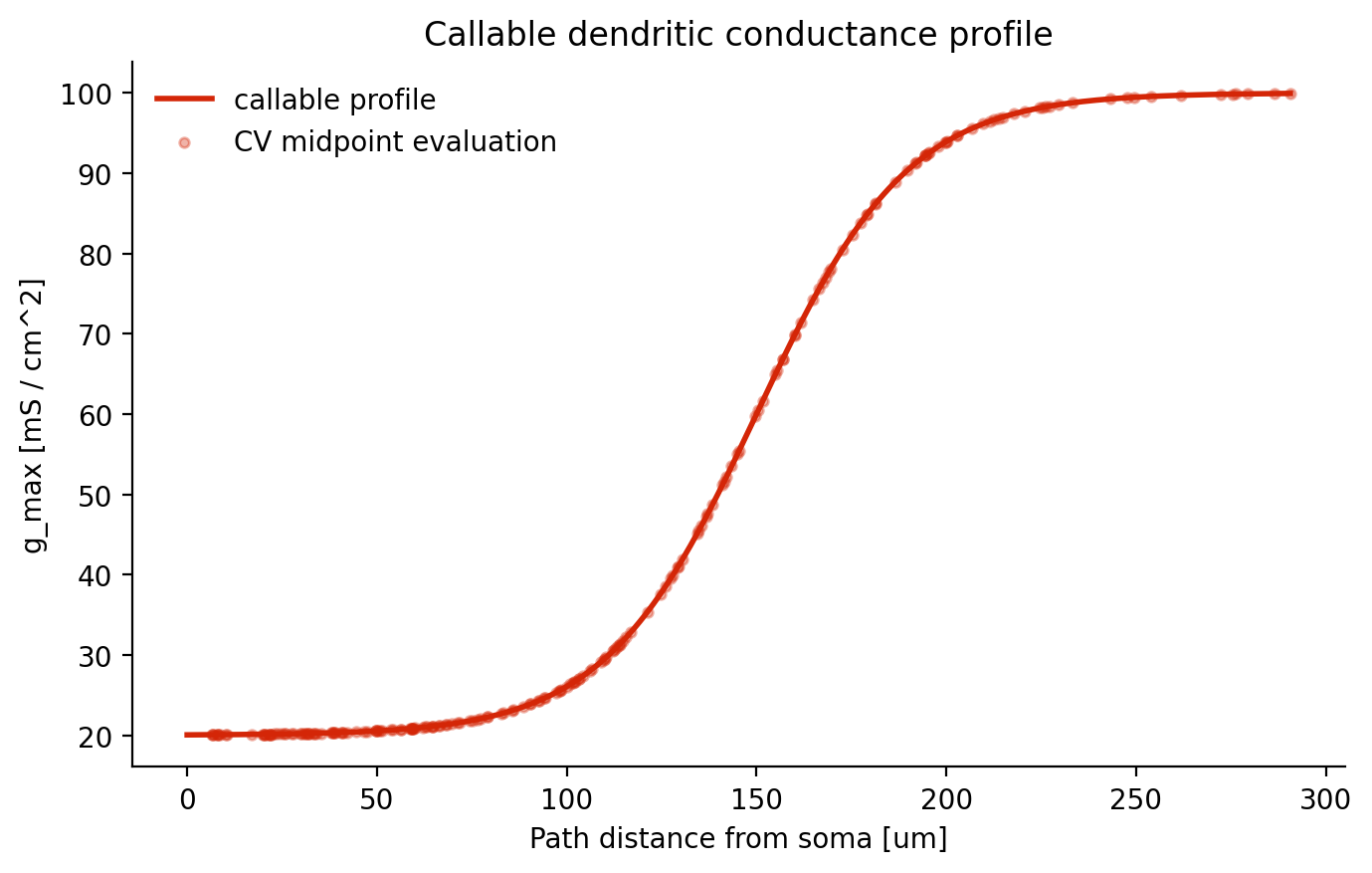
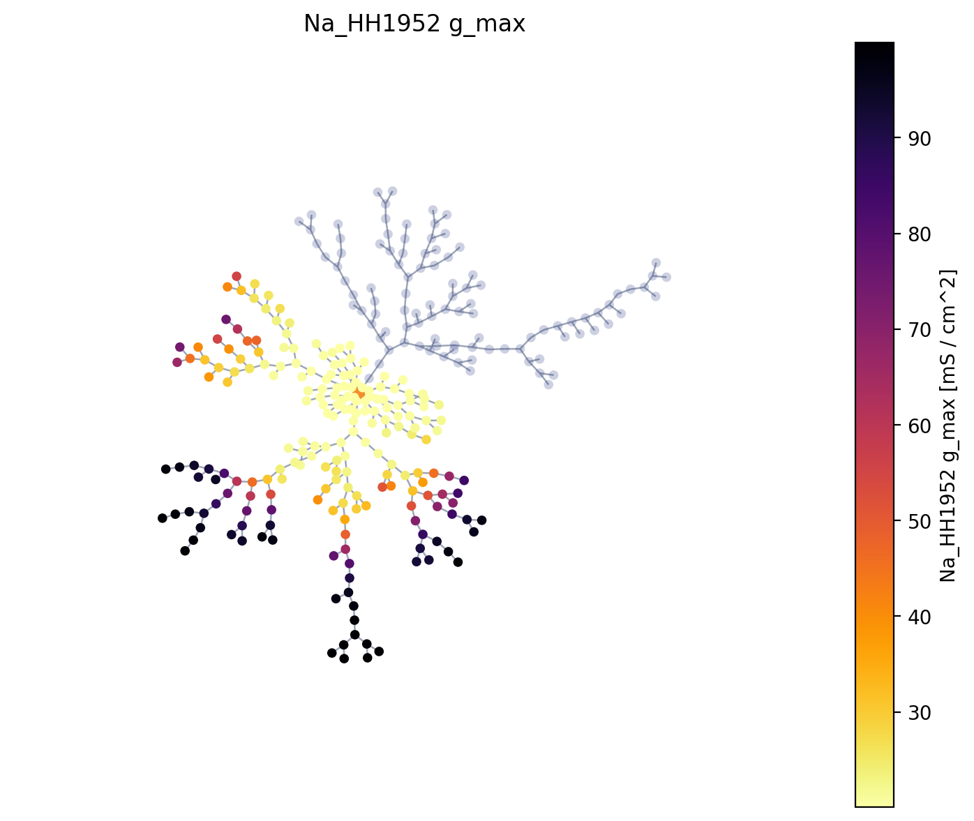
A density-mechanism parameter can be a callable instead of a constant. BrainCell passes a read-only CVContext to the callable and resolves it once per active CV during init_state(). Here, dendritic sodium conductance follows a sigmoid profile over path distance from the soma surface; the same callable declaration remains one runtime layout.

import numpy as np

G_MAX_UNIT = u.mS / u.cm**2

def gmax_from_distance(distance):
    distance_um = distance.to_decimal(u.um)
    return (20.0 + 0.15 * distance_um) * G_MAX_UNIT

def gmax_from_distance_sigmoid(distance):
    distance_um = distance.to_decimal(u.um)
    
    # 基础参数（可根据需要调整）
    g_min = 20.0    # 近端最小电导密度 (S/cm²)
    g_max = 100.0  # 远端最大电导密度 (S/cm²)
    d_0 = 150.0     # 半激活距离 (µm)，即密度上升到一半时的位置
    k = 0.05        # 陡峭度参数 (1/µm)，控制曲线上升的快慢
    
    g_value = g_min + (g_max - g_min) / (1 + np.exp(-k * (distance_um - d_0)))
    
    return g_value * G_MAX_UNIT

def dendritic_na_gmax(context):
    return gmax_from_distance_sigmoid(context.path_distance_from_soma)

distance_cell = Cell(goc, cv_policy=MaxCVLen(40 * u.um))
distance_cell.paint(
    AllRegion(),
    mech.Channel("IL", g_max=0.03 * G_MAX_UNIT, E=-70 * u.mV),
)
distance_cell.paint(
    dendrites,
    mech.Channel(
        "Na_HH1952",
        name="na_distance",
        g_max=dendritic_na_gmax,
    ),
)
distance_cell.init_state()

dendrite_contexts = [
    context
    for context in distance_cell.cv_contexts
    if context.branch_type == "dendrite"
]
print(f"callable evaluated on {len(dendrite_contexts)} dendritic CVs")

callable evaluated on 207 dendritic CVs

cv_distance_um = np.asarray([
    context.path_distance_from_soma.to_decimal(u.um)
    for context in dendrite_contexts
], dtype=float)
cv_gmax = np.asarray([
    dendritic_na_gmax(context).to_decimal(G_MAX_UNIT)
    for context in dendrite_contexts
], dtype=float)

distance_um = np.linspace(0.0, cv_distance_um.max(), 240)
curve_gmax = gmax_from_distance_sigmoid(distance_um * u.um).to_decimal(G_MAX_UNIT)
dendrite_color = vis.get_defaults().branch_type_colors["dendrite"]
if not isinstance(dendrite_color, str):
    dendrite_color = np.asarray(dendrite_color, dtype=float)
    if dendrite_color.max() > 1.0:
        dendrite_color = dendrite_color / 255.0

fig, ax = plt.subplots(figsize=(7, 4.5))
ax.plot(
    distance_um,
    curve_gmax,
    color=dendrite_color,
    linewidth=2.0,
    label="callable profile",
)
ax.scatter(
    cv_distance_um,
    cv_gmax,
    color=dendrite_color,
    s=12,
    alpha=0.35,
    label="CV midpoint evaluation",
)
ax.set_xlabel("Path distance from soma [um]")
ax.set_ylabel("g_max [mS / cm^2]")
ax.set_title("Callable dendritic conductance profile")
ax.legend(frameon=False)
fig.tight_layout()
curve_path = save_figure(fig, "gmax_callable_curve.png")
plt.close(fig)
display(Image(filename=curve_path))

fig, ax = plt.subplots(figsize=(8, 6))
distance_cell.vis_cv(
    value=("channel", "Na_HH1952", "g_max"),
    layout="kamada_kawai",
    cmap="inferno_r",
    vmin=float(cv_gmax.min()),
    vmax=float(cv_gmax.max()),
    value_label="Na_HH1952 g_max",
    ax=ax,
    show=False,
)

ax.set_title("Na_HH1952 g_max")
fig.tight_layout()
heatmap_path = save_figure(fig, "gmax_callable_dendrite_heatmap.png")
plt.close(fig)
display(Image(filename=heatmap_path))

Part 5 — Current interaction boundary

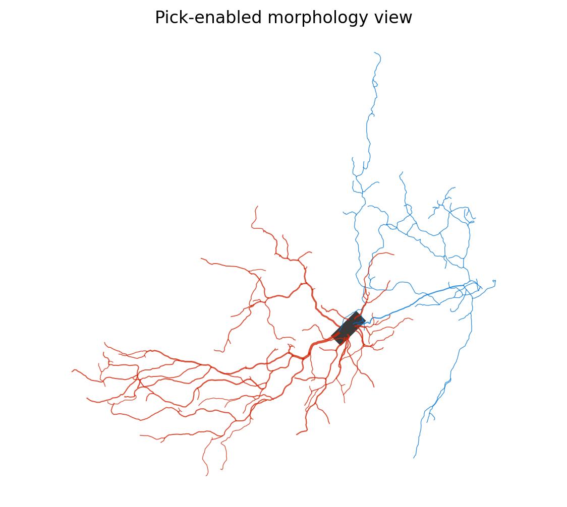
VisHooks already provides backend-independent pick, hover, and leave callbacks. With an interactive Matplotlib backend (for example %matplotlib widget) or PyVista picking, a callback receives branch identity, segment identity, fractional branch position, and the scene position. The cell below also executes under a non-interactive documentation backend; interaction begins when the notebook uses an interactive frontend.

def report_pick(info):
    print(info.branch_name, info.branch_type, info.segment_index, info.x)

hooks = vis.VisHooks(on_pick=report_pick)
fig, ax = plt.subplots(figsize=(7, 6))
vis.plot2d(goc, layout="projected", shape="line", hooks=hooks, ax=ax)
ax.set_title("Pick-enabled morphology view")
interaction_path = save_figure(fig, "interaction_entrypoint.png")
plt.close(fig)
display(Image(filename=interaction_path))
print("Pick callback registered; use an interactive backend to receive events.")

Pick callback registered; use an interactive backend to receive events.

Next interaction milestones

The event channel is present, but BrainCell does not yet provide a persistent editor. The next frontend work should preserve the programmatic model as the source of truth and add two explicit workflows:

1. Morphology editing — persistent multi-selection; insert, delete, move, and resize nodes or subtrees; validation; before/after comparison; undo/redo; and SWC/ASC or Python export. NeuroEditor is a direct reference for selection, correction, and before/after inspection. The TREES Toolbox is a mature reference for tree construction and manipulation.

2. Mechanism and synapse editing — synchronized morphology and topology views; visual RegionExpr/LocsetExpr construction; channel-parameter distributions; synapse placement; and export to paint/place declarations. DendroTweaks is the primary reference for linked views and interactive subcellular parameter distributions.

These are roadmap targets, not implemented APIs. The current executable boundary remains morphology ingestion, declarative selection and decoration, multi-level visualization, and event callbacks.