Mechanisms in BrainCell

Mechanisms in BrainCell#

This notebook now stays intentionally narrow.

Ion and Channel already have dedicated walkthroughs in 6.channel.ipynb and 7.ion.ipynb. Here we only keep the minimum density background needed to make point mechanisms concrete, then spend most of the notebook on probes.

At the declaration layer, the current multi-compartment mechanism surface still splits into two families:

Density: installed with cell.paint(region, ...)
Point: installed with cell.place(locset, ...)

CableProperty is closely related, but it is a passive cable declaration rather than a Mechanism subclass.

Family	Declaration	Attach with	What matters most	Coverage here
Passive cable declaration	`CableProperty`	`cell.paint(region, ...)`	Passive defaults such as `v_rest`, `cm`, `ra`, `temperature`	Short reminder
Density mech	`Ion`	`cell.paint(region, ...)`	Runtime ion containers and ion-side state	See `7.ion.ipynb`
Density mech	`Channel`	`cell.paint(region, ...)`	Distributed conductance mechanisms bound to ions	See `6.channel.ipynb`
Point mech	`CurrentClamp` / `SineClamp` / `FunctionClamp`	`cell.place(locset, ...)`	Current injection at point locations	Short refresher
Point mech	`StateProbe` / `MechanismProbe` / `CurrentProbe`	`cell.place(locset, ...)`	Read runtime state and current back out of the cell	Main focus
Point mech	`ProbeMechanism` / `Synapse` / `Junction`	`cell.place(locset, ...)`	Older or narrower workflows	Overview only

import os

os.environ.setdefault("JAX_PLATFORMS", "cpu")
os.environ.setdefault("MPLBACKEND", "Agg")

import brainunit as u
import matplotlib.pyplot as plt

from braincell import Branch, Cell, Morphology
from braincell.filter import AllRegion, BranchSlice, RootLocation, Terminals, at
from braincell.mech import (
    CableProperty,
    Channel,
    CurrentClamp,
    CurrentProbe,
    FunctionClamp,
    Ion,
    MechanismProbe,
    SineClamp,
    StateProbe,
)


def build_demo_morphology() -> Morphology:
    soma = Branch.from_lengths(
        lengths=[20.0] * u.um,
        radii=[8.0, 8.0] * u.um,
        type="soma",
    )
    dend = Branch.from_lengths(
        lengths=[60.0] * u.um,
        radii=[2.0, 1.2] * u.um,
        type="basal_dendrite",
    )
    axon = Branch.from_lengths(
        lengths=[80.0] * u.um,
        radii=[1.0, 0.6] * u.um,
        type="axon",
    )
    morpho = Morphology.from_root(soma, name="soma")
    morpho.attach(parent="soma", child_branch=dend, child_name="dend", parent_x=1.0)
    morpho.attach(parent="soma", child_branch=axon, child_name="axon", parent_x=0.0)
    return morpho

1. Density declarations: only the minimum background#

The density side has three layers:

CableProperty sets passive cable defaults.
Ion declares ion containers and any ion-side runtime state.
Channel installs distributed mechanisms that bind to those ions.

For the full density story, use the neighboring notebooks instead of this one:

4.cell.ipynb for the paint/place workflow on Cell
6.channel.ipynb for channel templates, gates, and generated ODEs
7.ion.ipynb for ion templates, Nernst handling, and dynamic ion state

That is enough context for probes, because probes only become interesting after Cell.init_state() has materialized runtime state from these declarations.

1.1 `CableProperty`: paintable, central, but passive#

CableProperty uses the same paint(...) entry point as density mechanisms, so it still belongs in the mental model even though it does not inherit from Mechanism.

morpho = build_demo_morphology()
print(morpho.topo())

cell_passive = Cell(morpho)
cell_passive.paint(
    AllRegion(),
    CableProperty(
        resting_potential=-65.0 * u.mV,
        membrane_capacitance=1.0 * (u.uF / u.cm**2),
        axial_resistivity=100.0 * (u.ohm * u.cm),
    ),
)

print()
print(cell_passive)
print("root CV resting potential:", cell_passive.cvs[0].v)

soma
├── dend
└── axon

Cell(root='soma', n_branches=3, n_paint_rules=1, n_place_rules=0, initialized=False)
root CV resting potential: -65. mV

2. Point mechanisms: stimuli versus observers#

Point mechanisms live at one location in the point tree rather than across a branch interval.

For this notebook, the useful split is:

stimuli: declarations that inject current at one point
observers: declarations that read runtime values back out of the cell

Locsets decide where those declarations land. If you want the full locset vocabulary, see 2.filter.ipynb.

2.1 Clamp declarations: a quick refresher#

CurrentClamp, SineClamp, and FunctionClamp all feed the same runtime path: cell.runtime.evaluate_point_clamps(t=...).

If several clamps are placed at the same point, their currents add. Since the rest of this notebook is probe-focused, we only keep one short runnable refresher here.

cell_clamp = Cell(build_demo_morphology())
cell_clamp.place(
    RootLocation(x=0.5),
    CurrentClamp(
        delay=0.0 * u.ms,
        durations=(2.0 * u.ms, 2.0 * u.ms),
        amplitudes=(0.0 * u.nA, 0.3 * u.nA),
    ),
    SineClamp(
        amplitude=0.2 * u.nA,
        frequency=500.0 * u.Hz,
        offset=0.1 * u.nA,
        duration=4.0 * u.ms,
    ),
    FunctionClamp(
        fn=lambda t: 0.4 * u.nA if t < 1.0 * u.ms else 0.0 * u.nA,
    ),
)
cell_clamp.init_state()

point_index = int(cell_clamp.layouts[0].point_index[0])
current_early = cell_clamp.runtime.evaluate_point_clamps(t=0.5 * u.ms)
current_late = cell_clamp.runtime.evaluate_point_clamps(t=2.5 * u.ms)

print("layout kinds:", [layout.kind for layout in cell_clamp.layouts])
print("active point index:", point_index)
print(f"combined clamp current at 0.5 ms: {float(current_early[point_index].to_decimal(u.nA)):.3f} nA")
print(f"combined clamp current at 2.5 ms: {float(current_late[point_index].to_decimal(u.nA)):.3f} nA")

layout kinds: ['CurrentClamp', 'SineClamp', 'FunctionClamp']
active point index: 1
combined clamp current at 0.5 ms: 0.700 nA
combined clamp current at 2.5 ms: 0.600 nA

2.2 Probes: the main observer surface#

Probes are sparse point declarations. They do not allocate their own evolving state; they sample state or current that already exists elsewhere in the initialized runtime.

The three public probe types are:

StateProbe: reads cell-owned state. In the current multi-compartment implementation, that means membrane voltage v.
MechanismProbe: reads a runtime state field from a named mechanism or ion.
CurrentProbe: reads the current of a named mechanism, or the total current of a named ion owner.

Once cell.init_state() has run, you can read probes in two ways:

cell.sample_probe(name) reads one probe snapshot by name.
cell.sample_probes() reads every probe snapshot as a {name: value} dictionary.

During time integration, cell.run(...) samples the same placed probes every timestep and returns them in RunResult.traces.

cell_probe = Cell(build_demo_morphology())
region = BranchSlice(branch_index=[0, 1], prox=0.0, dist=1.0)

cell_probe.paint(
    region,
    Channel("IL", g_max=0.03 * (u.mS / u.cm**2), E=-54.387 * u.mV),
    Channel("Na_HH1952", g_max=120.0 * (u.mS / u.cm**2)),
    Ion(
        "CalciumDetailed",
        name="ca_dyn",
        d=0.5 * u.um,
        tau=10.0 * u.ms,
        C_rest=5.0e-5 * u.mM,
        Ci_initializer=2.4e-4 * u.mM,
    ),
)
cell_probe.paint(
    BranchSlice(branch_index=0, prox=0.0, dist=1.0),
    Channel("CaT_HM1992", ion_name="ca_dyn", g_max=2.0 * (u.mS / u.cm**2)),
)

cell_probe.place(
    at("soma", 0.5),
    StateProbe(),
    MechanismProbe(mechanism="Na_HH1952", field="p"),
    MechanismProbe(mechanism="ca_dyn", field="Ci"),
    CurrentProbe(ion="na", mechanism="Na_HH1952"),
    CurrentProbe(ion="na"),
    CurrentProbe(mechanism="IL"),
)
cell_probe.init_state()

samples = cell_probe.sample_probes()

print("probe keys:", sorted(samples))
print("single lookup via sample_probe:", float(cell_probe.sample_probe("soma(0.5)_Na_HH1952_p")))
print("soma(0.5)_v (mV):", float(samples["soma(0.5)_v"].to_decimal(u.mV)))
print("soma(0.5)_Na_HH1952_p:", float(samples["soma(0.5)_Na_HH1952_p"]))
print("soma(0.5)_ca_dyn_Ci (mM):", float(samples["soma(0.5)_ca_dyn_Ci"].to_decimal(u.mM)))
print(
    "soma(0.5)_Na_HH1952_current (mA / cm^2):",
    float(samples["soma(0.5)_Na_HH1952_current"].to_decimal(u.mA / u.cm**2)),
)
print(
    "soma(0.5)_na_current (mA / cm^2):",
    float(samples["soma(0.5)_na_current"].to_decimal(u.mA / u.cm**2)),
)
print(
    "soma(0.5)_IL_current (mA / cm^2):",
    float(samples["soma(0.5)_IL_current"].to_decimal(u.mA / u.cm**2)),
)

probe keys: ['soma(0.5)_IL_current', 'soma(0.5)_Na_HH1952_current', 'soma(0.5)_Na_HH1952_p', 'soma(0.5)_ca_dyn_Ci', 'soma(0.5)_na_current', 'soma(0.5)_v']
single lookup via sample_probe: 0.0
soma(0.5)_v (mV): -65.0
soma(0.5)_Na_HH1952_p: 0.0
soma(0.5)_ca_dyn_Ci (mM): 0.00024
soma(0.5)_Na_HH1952_current (mA / cm^2): 0.0
soma(0.5)_na_current (mA / cm^2): 0.0
soma(0.5)_IL_current (mA / cm^2): 0.00031838996801525354

2.3 What can a probe measure, exactly?#

The practical rules are:

StateProbe(field="v") reads cell-owned membrane voltage. In the current implementation, v is the only supported state field.
MechanismProbe(mechanism="Na_HH1952", field="p") works well for channel gate variables and other runtime state stored as brainstate.State.
MechanismProbe also works on ion names, not only on channel names. That is why MechanismProbe(mechanism="ca_dyn", field="Ci") can read the dynamic calcium concentration created by Ion("CalciumDetailed", name="ca_dyn", ...).
Static parameters are not valid probe fields. For example, g_max is a parameter, not runtime state.
Derived properties are not valid probe fields either. For Nernst-style ions, E is computed from the current ion state; it is not stored as a standalone runtime State.
CurrentProbe(ion="na", mechanism="Na_HH1952") reads one mechanism current.
CurrentProbe(mechanism="IL") reads a mechanism current when the mechanism can evaluate current(...) without an explicit ion selector.
CurrentProbe(ion="na") reads the total current of the named ion owner.

In the snapshot above, soma(0.5)_Na_HH1952_current and soma(0.5)_na_current happen to match because only one sodium channel is present. Once several sodium channels share the same ion owner, the ion-total probe becomes their sum.

Probe names matter because every runtime lookup is name-keyed:

If you do not provide name=..., the lowerer auto-generates names such as soma(0.5)_v or soma(0.5)_Na_HH1952_p.
If you do provide name=..., it must still be globally unique. Duplicate names will make sample_probes() and run(...) ambiguous.

morpho_multi = build_demo_morphology()
locset = RootLocation(x=0.5) | Terminals()

cell_multi = Cell(morpho_multi)
cell_multi.place(locset, StateProbe())
cell_multi.init_state()

print("locset display names:", morpho_multi.select(locset).display_names)
print("resolved probe keys:", sorted(cell_multi.sample_probes()))
print()
for layout in cell_multi.layouts:
    declaration = cell_multi.runtime.get_layout_mechanism(layout.id)
    print(layout.kind, layout.point_index.tolist(), declaration.name)

locset display names: ('soma(0.5)', 'dend(1)', 'axon(1)')
resolved probe keys: ['axon(1)_v', 'dend(1)_v', 'soma(0.5)_v']

state_probe:v:soma(0.5)_v [1] soma(0.5)_v
state_probe:v:dend(1)_v [3] dend(1)_v
state_probe:v:axon(1)_v [5] axon(1)_v

A locset that resolves to several points therefore produces several probes, one per selected point, each with its own resolved name. That is usually what you want for sample_probes() and for RunResult.traces, because each trace stays keyed by one concrete point location.

2.4 `CurrentProbe` on mixed-ion channels: owner versus modulators#

Mixed-ion channels need one more piece of vocabulary.

Kca3p1_MA2020_GoC uses potassium as the current owner, while calcium acts as a modulator of the gating dynamics. In that case:

CurrentProbe(mechanism="Kca3p1_MA2020_GoC") asks the mechanism itself for its current, using all ions that were bound to it at runtime.
CurrentProbe(ion="k_main") asks the potassium owner for its total current, which may include several potassium channels.

To make that distinction visible, the example below adds a second potassium channel and briefly depolarizes the soma before comparing the two recorded currents.

cell_mixed = Cell(build_demo_morphology())
region = BranchSlice(branch_index=[0, 1], prox=0.0, dist=1.0)

cell_mixed.paint(
    region,
    Ion("PotassiumFixed", name="k_main", E=-88.0 * u.mV),
    Ion("CalciumFixed", name="ca_hva", Ci=2e-4 * u.mM),
    Ion("CalciumFixed", name="ca_lva", Ci=5e-4 * u.mM),
)
cell_mixed.paint(
    region,
    Channel("Kca3p1_MA2020_GoC", ion_names={"ca": "ca_hva"}),
    Channel("K_Kv_test", ion_name="k_main", g_max=1.0 * (u.mS / u.cm**2)),
)
cell_mixed.place(
    RootLocation(x=0.5),
    CurrentClamp(delay=0.5 * u.ms, durations=10.0 * u.ms, amplitudes=0.5 * u.nA),
)
cell_mixed.place(
    at("soma", 0.5),
    CurrentProbe(mechanism="Kca3p1_MA2020_GoC"),
    CurrentProbe(ion="k_main"),
)

result = cell_mixed.run(dt=0.05 * u.ms, duration=11.0 * u.ms)
layout = next(layout for layout in cell_mixed.layouts if layout.kind == "channel:Kca3p1_MA2020_GoC")
mech_trace = result.traces["soma(0.5)_Kca3p1_MA2020_GoC_current"].to_decimal(u.mA / u.cm**2)
total_trace = result.traces["soma(0.5)_k_main_current"].to_decimal(u.mA / u.cm**2)

print(sorted(result.traces))
print("bound ion keys:", cell_mixed.runtime.bound_ion_keys[layout.id])
print("current owner:", cell_mixed.runtime.current_owner_keys[layout.id])
print("last Kca mechanism current (mA / cm^2):", float(mech_trace[-1]))
print("last k_main total current (mA / cm^2):", float(total_trace[-1]))
print("difference at last timestep (mA / cm^2):", float(total_trace[-1] - mech_trace[-1]))

['soma(0.5)_Kca3p1_MA2020_GoC_current', 'soma(0.5)_k_main_current']
bound ion keys: ('k_main', 'ca_hva')
current owner: k_main
last Kca mechanism current (mA / cm^2): -0.022346971556544304
last k_main total current (mA / cm^2): -0.02325270138680935
difference at last timestep (mA / cm^2): -0.0009057298302650452

2.5 Probe traces during `cell.run(...)`#

Snapshots are useful when you want the value now. For a time series, you do not place a different declaration: you place the same probes and then call cell.run(...).

A few operational details matter:

cell.run(...) auto-calls init_state() if the cell is still in DECLARING.
cell.run(...) requires at least one placed probe, because its trace output is probe-driven.
The return value is RunResult(time=..., traces=...), where traces is a dictionary keyed by probe name.

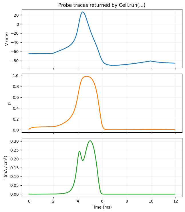
Below we drive the soma with a step current and record three traces from the same point: membrane voltage, one sodium gate variable, and the sodium mechanism current.

sim_cell = Cell(build_demo_morphology())
sim_region = BranchSlice(branch_index=[0, 1], prox=0.0, dist=1.0)

sim_cell.paint(
    sim_region,
    Channel("IL", g_max=0.03 * (u.mS / u.cm**2), E=-54.387 * u.mV),
    Channel("Na_HH1952", g_max=120.0 * (u.mS / u.cm**2)),
    Channel("K_HH1952", g_max=36.0 * (u.mS / u.cm**2)),
)

sim_cell.place(
    RootLocation(x=0.5),
    CurrentClamp(delay=2.0 * u.ms, durations=8.0 * u.ms, amplitudes=0.2 * u.nA),
)
sim_cell.place(
    at("soma", 0.5),
    StateProbe(),
    MechanismProbe(mechanism="Na_HH1952", field="p"),
    CurrentProbe(ion="na", mechanism="Na_HH1952"),
)

result = sim_cell.run(dt=0.05 * u.ms, duration=12.0 * u.ms)

print("trace keys:", sorted(result.traces))
print("n timesteps:", int(result.time.shape[0]))
print("current time after run (ms):", float(sim_cell.current_time.to_decimal(u.ms)))

fig, axes = plt.subplots(3, 1, figsize=(6.5, 7.5), sharex=True)

times_ms = result.time.to_decimal(u.ms)
axes[0].plot(times_ms, result.traces["soma(0.5)_v"].to_decimal(u.mV), color="#1f77b4", linewidth=2.0)
axes[0].set_ylabel("V (mV)")
axes[0].set_title("Probe traces returned by Cell.run(...)")
axes[0].grid(True, alpha=0.2)

axes[1].plot(times_ms, result.traces["soma(0.5)_Na_HH1952_p"], color="#ff7f0e", linewidth=2.0)
axes[1].set_ylabel("p")
axes[1].grid(True, alpha=0.2)

axes[2].plot(
    times_ms,
    result.traces["soma(0.5)_Na_HH1952_current"].to_decimal(u.mA / u.cm**2),
    color="#2ca02c",
    linewidth=2.0,
)
axes[2].set_xlabel("Time (ms)")
axes[2].set_ylabel("I (mA / cm$^2$)")
axes[2].grid(True, alpha=0.2)

plt.tight_layout()
plt.show()

trace keys: ['soma(0.5)_Na_HH1952_current', 'soma(0.5)_Na_HH1952_p', 'soma(0.5)_v']
n timesteps: 240
current time after run (ms): 12.0

../_images/516823d97a4783ee691b0bfc6b1b540ed777097423f17dd44e4f167326b8c407.png

2.6 Other point declarations#

Three public point declarations are worth knowing even though this notebook does not build their full workflows.

ProbeMechanism(variable="v", target="soma") is the older variable-by-name recorder. For new multi-compartment code, prefer StateProbe, MechanismProbe, and CurrentProbe when you want explicit selectors.
Synapse(synapse_type="AMPA", ...) is the registry-keyed synapse declaration surface.
Junction(...) is the current placeholder for gap-junction-style point declarations.

Summary#

The mechanism surface in the current multi-compartment stack is still small, but the probe story is already quite usable:

CableProperty, Ion, and Channel create the runtime objects that probes later observe.
StateProbe is the voltage probe: today it supports only v.
MechanismProbe reads named runtime state on a channel or ion, as long as the field is a real runtime State.
CurrentProbe can read one mechanism current or one ion owner’s total current.
cell.sample_probe(...) and cell.sample_probes() give immediate snapshots after init_state().
cell.run(...) records the same placed probes over time and returns them by probe name in RunResult.traces.

For more declaration detail, continue with 6.channel.ipynb and 7.ion.ipynb. For more locset detail, continue with 2.filter.ipynb.

Mechanisms in BrainCell

Contents

Mechanisms in BrainCell#

1. Density declarations: only the minimum background#

1.1 `CableProperty`: paintable, central, but passive#

2. Point mechanisms: stimuli versus observers#

2.1 Clamp declarations: a quick refresher#

2.2 Probes: the main observer surface#

2.3 What can a probe measure, exactly?#

2.4 `CurrentProbe` on mixed-ion channels: owner versus modulators#

2.5 Probe traces during `cell.run(...)`#

2.6 Other point declarations#

Summary#

Modeling

Infrastructure

Compilation

Mechanisms in BrainCell

Contents

Mechanisms in BrainCell#

1. Density declarations: only the minimum background#

1.1 CableProperty: paintable, central, but passive#

2. Point mechanisms: stimuli versus observers#

2.1 Clamp declarations: a quick refresher#

2.2 Probes: the main observer surface#

2.3 What can a probe measure, exactly?#

2.4 CurrentProbe on mixed-ion channels: owner versus modulators#

2.5 Probe traces during cell.run(...)#

2.6 Other point declarations#

Summary#

1.1 `CableProperty`: paintable, central, but passive#

2.4 `CurrentProbe` on mixed-ion channels: owner versus modulators#

2.5 Probe traces during `cell.run(...)`#