
How to add short-term plasticity#
Task. Model use-dependent synapses whose efficacy changes on a fast
timescale — short-term facilitation (STP) and short-term depression (STD).
Audience. Simulation. Assumes Tutorial 2 · Synapses and projections.
Short-term plasticity makes a synapse’s strength depend on its recent activity.
brainpy.state provides two models you can drive directly:
STP— the Tsodyks–Markram model with both facilitation and depression, tracking a utilization variableuand a resources variablex. The effective release is proportional tou · x.STD— pure depression, tracking the resourcesx.
Here we examine their dynamics in isolation: drive each with a regular spike train and watch the internal variables and the resulting efficacy evolve. This is the clearest way to understand what each model does before wiring it into a projection.
import brainpy
import brainstate
import braintools
import brainunit as u
import matplotlib.pyplot as plt
An NVIDIA GPU may be present on this machine, but a CUDA-enabled jaxlib is not installed. Falling back to cpu.
A regular presynaptic spike train#
We build a 20 Hz spike train over 400 ms (one spike every 50 ms).
with brainstate.environ.context(dt=0.1 * u.ms):
    times = u.math.arange(0. * u.ms, 400. * u.ms, brainstate.environ.get_dt())
    t_ms = times.to_decimal(u.ms)
    # a spike whenever the time is (almost) a multiple of 50 ms
    spike_train = (u.math.asarray((t_ms % 50.0) < 0.05)).astype(float)
Short-term facilitation + depression (STP)#
STP.update(pre_spike) advances u and x and returns the modulated efficacy.
With a long facilitation time constant, u ramps up across the train while x
is drawn down — the product u·x shows the net synaptic efficacy.
with brainstate.environ.context(dt=0.1 * u.ms):
    stp = brainpy.state.STP(1, U=0.2, tau_f=1500. * u.ms, tau_d=200. * u.ms)
    brainstate.nn.init_all_states(stp)

    def step_stp(sp):
        eff = stp(sp)
        return eff, stp.u.value, stp.x.value

    eff_stp, u_var, x_var = brainstate.transform.for_loop(step_stp, spike_train)

fig, gs = braintools.visualize.get_figure(2, 1, 1.8, 7.0)
ax = fig.add_subplot(gs[0, 0])
ax.plot(t_ms, u_var[:, 0], label='u (facilitation)')
ax.plot(t_ms, x_var[:, 0], label='x (resources)')
ax.legend(loc='center right'); ax.set_ylabel('STP variables')
ax = fig.add_subplot(gs[1, 0])
ax.plot(t_ms, (u_var * x_var)[:, 0], color='k')
ax.set_ylabel('efficacy u*x'); ax.set_xlabel('Time (ms)')
plt.show()

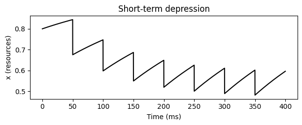
Short-term depression (STD)#
STD tracks only the resources x, which deplete with each spike and recover
with time constant tau. Successive spikes in the train produce progressively
weaker responses.
with brainstate.environ.context(dt=0.1 * u.ms):
    std = brainpy.state.STD(1, tau=200. * u.ms, U=0.2)
    brainstate.nn.init_all_states(std)

    def step_std(sp):
        eff = std(sp)
        return eff, std.x.value

    eff_std, x_std = brainstate.transform.for_loop(step_std, spike_train)

plt.figure(figsize=(7, 2.2))
plt.plot(t_ms, x_std[:, 0], color='k')
plt.ylabel('x (resources)'); plt.xlabel('Time (ms)')
plt.title('Short-term depression')
plt.show()
Using STP/STD in a projection#
To make a projection dynamic, the functional projection builders accept an
stp= describer, e.g.::
brainpy.state.align_post_projection(
    pre.prefetch('V'),
    lambda v: pre.get_spike(v) != 0.,
    comm=brainstate.nn.EventFixedProb(n_pre, n_post, 0.1, w),
    syn=brainpy.state.Expon.desc(n_post, tau=5. * u.ms),
    out=brainpy.state.COBA.desc(E=0. * u.mV),
    post=post,
    stp=brainpy.state.STP.desc(n_pre, U=0.2, tau_f=1500. * u.ms, tau_d=200. * u.ms),
)
See also#
BrainPy-style Plasticity —
STPandSTDreference.How to add synaptic delays — add transmission delays to a projection.
AlignPre / AlignPost — the keystone — how projections route presynaptic state.