
5-minute tour#
Who it’s for: everyone — this single example serves both worlds. Computational neuroscientists get a working spiking network; brain-inspired-computing readers get the exact same model that is later trained with gradients.
What you’ll learn: how to build an excitatory–inhibitory (E/I) balanced network, run it efficiently with brainstate.transform, and plot a spike raster — the “aha” that shows what brainpy.state does.
Imports#
Everything comes from the public ecosystem surface: brainpy.state for the models, brainstate for state + compilation, braintools for initializers, and brainunit for physical units.
import brainpy
import brainstate
import braintools
import brainunit as u
import matplotlib.pyplot as plt
An NVIDIA GPU may be present on this machine, but a CUDA-enabled jaxlib is not installed. Falling back to cpu.
The model: a COBA E/I network#
We build the classic conductance-based (COBA) balanced network of Vogels & Abbott (2005) / Brette et al. (2007): 3200 excitatory and 800 inhibitory leaky integrate-and-fire neurons, sparsely and recurrently connected.
Notice the structure of each projection — this is the keystone AlignPost design (AlignPostProj), built from four roles:
comm— the connection matrix (here a sparse event-driven connectivity,EventFixedProb),syn— the synapse dynamics (Expon.desc, an exponential synapse describer),out— how the synapse drives the target (COBA.desc, conductance-based),post— the postsynaptic population.
We cover why this shape matters in the keystone chapter.
class EINet(brainstate.nn.Module):
    def __init__(self):
        super().__init__()
        self.n_exc, self.n_inh = 3200, 800
        self.num = self.n_exc + self.n_inh
        # One shared population of refractory LIF neurons.
        self.N = brainpy.state.LIFRef(
            self.num,
            V_rest=-60. * u.mV, V_th=-50. * u.mV, V_reset=-60. * u.mV,
            tau=20. * u.ms, tau_ref=5. * u.ms,
            V_initializer=braintools.init.Normal(-55., 2., unit=u.mV),
        )
        # Excitatory projection (reversal potential 0 mV).
        self.E = brainpy.state.AlignPostProj(
            comm=brainstate.nn.EventFixedProb(
                self.n_exc, self.num, conn_num=0.02, conn_weight=0.6 * u.mS),
            syn=brainpy.state.Expon.desc(self.num, tau=5. * u.ms),
            out=brainpy.state.COBA.desc(E=0. * u.mV),
            post=self.N,
        )
        # Inhibitory projection (reversal potential -80 mV).
        self.I = brainpy.state.AlignPostProj(
            comm=brainstate.nn.EventFixedProb(
                self.n_inh, self.num, conn_num=0.02, conn_weight=6.7 * u.mS),
            syn=brainpy.state.Expon.desc(self.num, tau=10. * u.ms),
            out=brainpy.state.COBA.desc(E=-80. * u.mV),
            post=self.N,
        )

    def update(self, t, inp):
        with brainstate.environ.context(t=t):
            spk = self.N.get_spike() != 0.
            self.E(spk[:self.n_exc])   # route excitatory spikes
            self.I(spk[self.n_exc:])   # route inhibitory spikes
            self.N(inp)                # advance neurons one step
            return self.N.get_spike()
Build and initialize#
Constructing the module allocates its parameters; brainstate.nn.init_all_states then allocates and resets every dynamic state (membrane potentials, synaptic conductances) so the network is ready to run.
net = EINet()
brainstate.nn.init_all_states(net)
EINet(
  n_exc=3200,
  n_inh=800,
  num=4000,
  N=LIFRef(
    in_size=(4000,),
    out_size=(4000,),
    before_updates={
      "(<class 'brainpy.state.Expon'>, (4000,), {'tau': '5. ms'}) // (<class 'brainpy.state.COBA'>, (), {'E': '0. mV'})": _AlignPost(
        syn=Expon(
          in_size=(4000,),
          out_size=(4000,),
          tau=Quantity(5., "ms"),
          g_initializer=Constant(value=0. mS),
          g=HiddenState(
            value=Quantity(~float32[4000], "mS")
          )
        ),
        out=COBA(
          E=Quantity(0., "mV")
        )
      ),
      "(<class 'brainpy.state.Expon'>, (4000,), {'tau': '10. ms'}) // (<class 'brainpy.state.COBA'>, (), {'E': '-80. mV'})": _AlignPost(
        syn=Expon(
          in_size=(4000,),
          out_size=(4000,),
          tau=Quantity(10., "ms"),
          g_initializer=Constant(value=0. mS),
          g=HiddenState(
            value=Quantity(~float32[4000], "mS")
          )
        ),
        out=COBA(
          E=Quantity(-80., "mV")
        )
      )
    },
    current_inputs={
      'AlignPostProj0': COBA(...),
      'AlignPostProj1': COBA(...)
    },
    spk_reset=soft,
    spk_fun=ReluGrad(alpha=0.3, width=1.0),
    R=Quantity(1., "ohm"),
    tau=Quantity(20., "ms"),
    tau_ref=Quantity(5., "ms"),
    V_th=Quantity(-50., "mV"),
    V_rest=Quantity(-60., "mV"),
    V_reset=Quantity(-60., "mV"),
    V_initializer=Normal(mean=-55.0, std=2.0),
    V=HiddenState(
      value=Quantity(float32[4000], "mV")
    ),
    last_spike_time=ShortTermState(
      value=Quantity(~float32[4000], "ms")
    )
  ),
  E=AlignPostProj(
    name=AlignPostProj0,
    modules=(),
    merging=True,
    comm=EventFixedNumConn(
      in_size=(3200,),
      out_size=(4000,),
      efferent_target=post,
      conn_num=80,
      allow_multi_conn=True,
      weight=ParamState(
        value=Quantity(~float32[], "mS")
      ),
      conn=FixedNumPerPre(float32[3200, 4000], nse=256000)
    ),
    syn=Expon(...),
    out=COBA(...),
    post=LIFRef(...)
  ),
  I=AlignPostProj(
    name=AlignPostProj1,
    modules=(),
    merging=True,
    comm=EventFixedNumConn(
      in_size=(800,),
      out_size=(4000,),
      efferent_target=post,
      conn_num=80,
      allow_multi_conn=True,
      weight=ParamState(
        value=Quantity(~float32[], "mS")
      ),
      conn=FixedNumPerPre(float32[800, 4000], nse=64000)
    ),
    syn=Expon(...),
    out=COBA(...),
    post=LIFRef(...)
  )
)
Run the simulation#
We advance the network for 1000 ms with a constant external drive.
We never step the model with a bare Python for loop. brainstate.transform.for_loop lowers the entire time loop into a single compiled XLA program — the body is traced once, fused, and the per-step outputs are stacked for you. (For other shapes of work use scan, jit, or the checkpointed_* variants.)
with brainstate.environ.context(dt=0.1 * u.ms):
    times = u.math.arange(0. * u.ms, 1000. * u.ms, brainstate.environ.get_dt())
    spikes = brainstate.transform.for_loop(
        lambda t: net.update(t, 20. * u.mA), times)
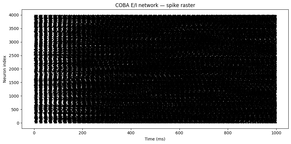
Visualize: a spike raster#
spikes has shape [time, neuron]. We find where spikes occurred and scatter neuron index against time.
t_idx, n_idx = u.math.where(spikes)
plt.figure(figsize=(10, 5))
plt.scatter(times[t_idx].to_decimal(u.ms), n_idx, s=1, color='black')
plt.xlabel('Time (ms)')
plt.ylabel('Neuron index')
plt.title('COBA E/I network — spike raster')
plt.tight_layout()
plt.show()
See also#
Core Concepts — the Core Concepts spine: why this design works, ending in the keystone AlignPre/AlignPost chapter.
The mental model — the four big ideas behind the code you just ran.
BrainPy-style Modeling — go deeper with the BrainPy-style tutorials and how-to guides, including the E/I network tutorial.