The state paradigm

What you’ll learn / who it’s for (simulation and training). Why a functional array library like JAX needs an explicit notion of state, how brainpy.state provides it, and how to advance a model through time the right way — never with a bare Python loop. Everything else in the documentation builds on these primitives.

The problem: dynamics without mutable variables

A spiking network is state evolving in time: membrane potentials, synaptic conductances, eligibility traces. But JAX — the engine underneath brainpy.state — is functional. Its arrays are immutable, and its real power (jit compilation, grad automatic differentiation, vmap batching) comes from transforming pure functions that take values in and return values out.

Threading every hidden variable through every function call by hand would be unbearable for anything larger than a single neuron. brainstate.State resolves the tension: state is held in explicit, trackable containers, so your model code reads imperatively, while the framework still hands JAX the pure functions it needs. (brainpy.state is the point-neuron layer built on brainstate; the two names appear side by side throughout.)

import brainpy
import brainstate
import braintools
import brainunit as u
import jax.numpy as jnp
import matplotlib.pyplot as plt

An NVIDIA GPU may be present on this machine, but a CUDA-enabled jaxlib is not installed. Falling back to cpu.

State: a trackable, differentiable variable

A State wraps a value (almost always a JAX array, usually carrying physical units) and exposes it through .value. You read and write .value like an ordinary attribute, but because the container is tracked, the framework can collect it, batch it, checkpoint it, and route gradients through it.

# A scalar state and a matrix state.
voltage = brainstate.State(-65.0 * u.mV)
weights = brainstate.State(jnp.array([[0.1, 0.2], [0.3, 0.4]]))

# Read and update through .value
print(voltage.value)
voltage.value = voltage.value + 5.0 * u.mV
print(voltage.value)

-65. mV
-60. mV

State types carry intent

brainpy.state distinguishes states by role, and transformations key off the distinction:

• ParamState — trainable parameters (weights, learnable time constants). brainstate.transform.grad differentiates with respect to these.

• ShortTermState / HiddenState — dynamical variables that evolve every step (membrane potential, conductance) and are reset between runs.

You rarely create these by hand — the built-in neurons and synapses declare them for you — but knowing the split explains how training selects exactly the right variables:

class LeakyUnit(brainstate.nn.Module):
    def __init__(self, size, tau=10.0 * u.ms):
        super().__init__()
        self.tau = brainstate.ParamState(tau)              # trainable
        self.v = brainstate.ShortTermState(jnp.zeros(size) * u.mV)  # dynamical

    def update(self, x):
        dt = brainstate.environ.get_dt()
        self.v.value = self.v.value + (-self.v.value + x) / self.tau.value * dt
        return self.v.value

init_all_states: allocate the dynamical variables

A freshly constructed model knows its parameters but has not yet allocated its dynamical state — that depends on the batch size you want to run. One call walks the whole module tree and initializes every state:

neuron = brainpy.state.LIF(
    100,
    V_rest=-65. * u.mV, V_th=-50. * u.mV, V_reset=-65. * u.mV,
    tau=10. * u.ms,
)

# Allocate states for a single trial ...
brainstate.nn.init_all_states(neuron)
print('unbatched V shape:', neuron.V.value.shape)

# ... or for a batch of 32 trials run in parallel.
brainstate.nn.init_all_states(neuron, batch_size=32)
print('batched   V shape:', neuron.V.value.shape)

unbatched V shape: (100,)
batched   V shape: (32, 100)

Call init_all_states again whenever you want to reset the model — for example at the start of every training epoch, so each minibatch starts from a clean slate (you’ll see exactly this in Differentiability).

environ.context: the simulation clock

Discrete-time dynamics need a time step dt (and often the current time t). Rather than thread these through every call, brainpy.state reads them from a context manager. Set dt once around your run; set t inside the per-step function so time-dependent inputs and synapses see the right value.

with brainstate.environ.context(dt=0.1 * u.ms):
    print('dt =', brainstate.environ.get_dt())
    # A per-step update would set t as well:
    with brainstate.environ.context(t=3.0 * u.ms):
        print('t  =', brainstate.environ.get('t'))

dt = 0.1 ms
t  = 3. ms

Driving a model: use transform, never a bare Python loop

This is the single most important runtime rule in brainpy.state.

A Python for/while loop over time steps executes op by op: each iteration pays Python dispatch overhead, nothing fuses, and under autodiff the body is re-traced on every step. The brainstate.transform primitives instead lower the entire loop into one compiled XLA program, tracing the body once. The speed-up is typically one to two orders of magnitude, and it is the difference between a model that trains and one that does not.

Pick the primitive by the shape of the work:

• Single step / one-shot call → brainstate.transform.jit — compile once, reuse the trace.

• Many steps, collect outputs → brainstate.transform.for_loop — repeat a step length times or map over xs; State is carried automatically and stacked outputs are returned.

• Many steps with an explicit carry → brainstate.transform.scan — thread a carry value alongside State (f(carry, x) -> (carry, y)).

• Long rollout under autograd (BPTT) → brainstate.transform.checkpointed_for_loop / checkpointed_scan — same semantics, but rematerialize activations on the backward pass to bound peak memory at the cost of recomputation.

Compose them freely (e.g. jit an outer driver that calls a for_loop). An outer optimization/epoch loop in plain Python is fine — the rule is about time-stepping the model.

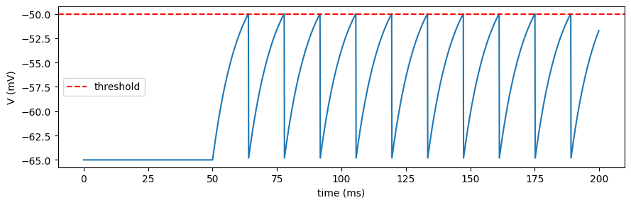
for_loop in action

Inject a step current into a single LIF neuron and collect its voltage trace. The step function sets t and returns what we want stacked over time; for_loop handles the rest.

neuron = brainpy.state.LIF(
    1,
    V_rest=-65. * u.mV, V_th=-50. * u.mV, V_reset=-65. * u.mV,
    tau=10. * u.ms, spk_reset='hard',
)
brainstate.nn.init_all_states(neuron)

def step(t):
    with brainstate.environ.context(t=t):
        current = u.math.where(t > 50. * u.ms, 20. * u.mA, 0. * u.mA)
        neuron(jnp.ones(1) * current)
        return neuron.V.value

with brainstate.environ.context(dt=0.1 * u.ms):
    times = u.math.arange(0. * u.ms, 200. * u.ms, brainstate.environ.get_dt())
    voltages = brainstate.transform.for_loop(step, times)

plt.figure(figsize=(9, 3))
plt.plot(times.to_decimal(u.ms), voltages.to_decimal(u.mV).squeeze())
plt.axhline(-50, color='r', ls='--', label='threshold')
plt.xlabel('time (ms)'); plt.ylabel('V (mV)'); plt.legend(); plt.tight_layout()
plt.show()

jit for a single compiled call

When you call the same step repeatedly from your own outer logic, wrap it in jit so it compiles once and every subsequent call is fast:

@brainstate.transform.jit
def one_step(current):
    neuron(current)
    return neuron.get_spike()

brainstate.nn.init_all_states(neuron)
with brainstate.environ.context(dt=0.1 * u.ms, t=0. * u.ms):
    _ = one_step(jnp.ones(1) * 20. * u.mA)   # first call compiles
    _ = one_step(jnp.ones(1) * 20. * u.mA)   # subsequent calls are fast

Recap

• A model is state evolving in time; brainstate.State makes that state explicit and visible to JAX’s transformations.

• init_all_states allocates (and resets) dynamical variables, optionally batched.

• environ.context supplies dt and t.

• Drive models with transform (jit / for_loop / scan / checkpointed_*) — never a bare Python loop over time steps.

See also

• Physical units — the unit system every state carries.

• Model anatomy — the Dynamics contract these states live in.

• AlignPre / AlignPost — the keystone — the keystone projection design.

• Differentiability — for_loop and checkpointed_* under grad for training.