
Connect a network#
What you’ll learn / who it’s for (simulation). NEST-like wiring with connection rules, assembled into a small Brunel (2000) random balanced network — the canonical sparse E/I network. We use delta synapses (iaf_psc_delta), so weights are membrane-voltage jumps in mV.
We keep order small here so the notebook runs fast; the example gallery has full-scale Brunel variants. Ported from examples/nest_like/brunel_delta.py.
import jax
jax.config.update('jax_enable_x64', True)
import brainstate
brainstate.environ.set(precision=64)

import numpy as np
import brainunit as u
import braintools
import matplotlib.pyplot as plt
from brainpy import state as bp
An NVIDIA GPU may be present on this machine, but a CUDA-enabled jaxlib is not installed. Falling back to cpu.
Brunel parameters#
The standard Brunel knobs: g (relative inhibition), eta (external drive relative to threshold), epsilon (connection density). NE/NI are the population sizes and CE/CI the in-degrees. We pick a small order for a quick run.
order = 100                         # small for a fast notebook run
g, eta, epsilon = 5.0, 2.0, 0.1
delay = 1.5                         # ms
NE, NI = 4 * order, 1 * order
CE, CI = int(epsilon * NE), int(epsilon * NI)
N_rec = 50
tauMem, CMem, theta, tref = 20.0, 1.0, 20.0, 2.0

J = 0.1                             # mV, delta postsynaptic jump
J_ex = J
J_in = -g * J_ex
nu_th = theta / (J * CE * tauMem)
p_rate = 1000.0 * (eta * nu_th) * CE   # external Poisson rate (Hz)
Create populations and the external drive#
Two iaf_psc_delta populations and a poisson_generator background. Each population also gets a spike_recorder tapping the first N_rec neurons.
npar = dict(C_m=CMem * u.pF, tau_m=tauMem * u.ms, t_ref=tref * u.ms,
            E_L=0. * u.mV, V_reset=0. * u.mV, V_th=theta * u.mV,
            V_initializer=braintools.init.Constant(0. * u.mV))

sim = bp.Simulator(dt=0.1 * u.ms)
ne = sim.create(bp.iaf_psc_delta, NE, params=npar)
ni = sim.create(bp.iaf_psc_delta, NI, params=npar)
noise = sim.create(bp.poisson_generator, rate=p_rate * u.Hz)
esr = sim.create(bp.spike_recorder)
isr = sim.create(bp.spike_recorder)
Wire the network with connection rules#
The background drives every neuron:
rule=all_to_all.Recurrent excitation and inhibition use
fixed_indegree(K)— each target drawsKrandom presynaptic partners (the Brunel rule).comm='sparse'keeps the event communication memory-light;seed=makes the draw reproducible.ne + nitargets the whole network in one call;ne[:N_rec]records a sub-sample.
sim.connect(noise, ne, weight=J_ex * u.mV, delay=delay * u.ms, rule=bp.all_to_all)
sim.connect(noise, ni, weight=J_ex * u.mV, delay=delay * u.ms, rule=bp.all_to_all)
sim.connect(ne, ne + ni, weight=J_ex * u.mV, delay=delay * u.ms,
            rule=bp.fixed_indegree(CE), comm='sparse', allow_multapses=True, seed=1)
sim.connect(ni, ne + ni, weight=J_in * u.mV, delay=delay * u.ms,
            rule=bp.fixed_indegree(CI), comm='sparse', allow_multapses=True, seed=2)
sim.connect(ne[:N_rec], esr)
sim.connect(ni[:N_rec], isr)

res = sim.simulate(1000. * u.ms)
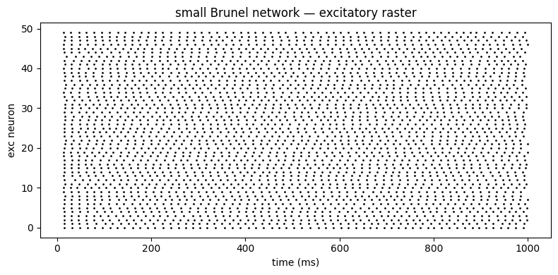
Firing rates and the excitatory raster#
erate = res.rate(esr.segments[0].population)
irate = res.rate(isr.segments[0].population)
print(f'excitatory rate: {erate:.2f} spks/s')
print(f'inhibitory rate: {irate:.2f} spks/s')

spk = np.asarray(res.spikes(esr.segments[0].population))   # (T, N_rec)
ts, ids = np.nonzero(spk > 0)
plt.figure(figsize=(8, 4))
plt.scatter(ts * 0.1, ids, s=1.0, color='k')
plt.xlabel('time (ms)'); plt.ylabel('exc neuron')
plt.title('small Brunel network — excitatory raster')
plt.tight_layout()
excitatory rate: 60.56 spks/s
inhibitory rate: 60.18 spks/s
See also#
Connectivity — connection rules and the synapse spec.
Porting walkthrough — Brunel side by side with NEST.
Example gallery — full-scale Brunel and other networks.
Validation status — how network parity is asserted (distributional, category D).