AlignPre / AlignPost — the keystone

What you’ll learn / who it’s for (simulation and training). This is the central design of brainpy.state and the single most important page in this documentation. You’ll learn why a naive simulator drowns in synaptic state, how AlignPre and AlignPost reduce that state from per-synapse to per-neuron — exactly, not approximately — the four components every projection is built from, and a decision table for choosing between the two. The chapter closes on the reason this matters twice over: the same alignment that makes simulation memory-efficient is what makes gradient-based and online learning memory-efficient.

A deep-learning reader can read “synapse” as “the recurrent hidden state of a layer”; a neuroscience reader can read it literally. Both arrive at the same place.

1. The synaptic-state explosion

Give every synapse its own dynamical variable and the bookkeeping grows with the number of connections. For a projection from \(N_{\text{pre}}\) to \(N_{\text{post}}\) neurons at connection density \(p\), naive per-synapse state costs

\[\mathcal{O}\!\left(p \cdot N_{\text{pre}} \cdot N_{\text{post}}\right).\]

Make it concrete. A modest cortical column might wire \(10^4\) neurons to \(10^4\) neurons at \(10\%\) density. That is \(\approx 10^7\) real synapses — but a naive implementation that materializes a variable for every possible pre–post pair allocates on the order of \(10^8\) floats, and updates all of them every step. Most of that is wasted: synapses that share dynamics are tracked redundantly.

The fix is not to approximate the dynamics. It is to notice that the redundancy is exact, and to store one variable where many identical ones used to live.

2. The key observation

All synaptic variables sharing the same linear dynamics can be reduced to a single one.

If a group of synapses obey the same differential equation and are driven by the same input, their states are identical for all time — so one state suffices for the whole group. The only question is which dimension the surviving variable should live on. Align it to the presynaptic neurons and you get AlignPre; align it to the postsynaptic neurons and you get AlignPost. Each is exact under a clearly stated condition, and each is natural for a different connectivity shape.

3. Decoupling dynamics from communication — the four roles

brainpy.state does not write projections as monolithic connection objects. Every projection is composed from four interchangeable roles, and the order of two of them is what distinguishes the two alignments:

• comm — communication. The connectivity itself: a sparse or dense weight matrix, or, equivalently, a deep-learning layer (EventFixedProb, Linear, AllToAllProj, …). It maps a presynaptic signal to a postsynaptic one.

• syn — synapse dynamics. The temporal filter applied to spikes (Expon, DualExpon, AMPA, GABAa, BioNMDA, …).

• out — output. How conductance becomes current: COBA (conductance- based, with reversal potential E), CUBA (current-based), or MgBlock (NMDA’s voltage-dependent magnesium block).

• post — the postsynaptic Dynamics population that receives the current.

Because the roles are decoupled, you swap connectivity, kinetics, and biophysics independently — and you place syn either before comm (AlignPre) or after it (AlignPost). That single placement choice is the whole idea, and the diagram below is the picture to hold in your head for the rest of the page.

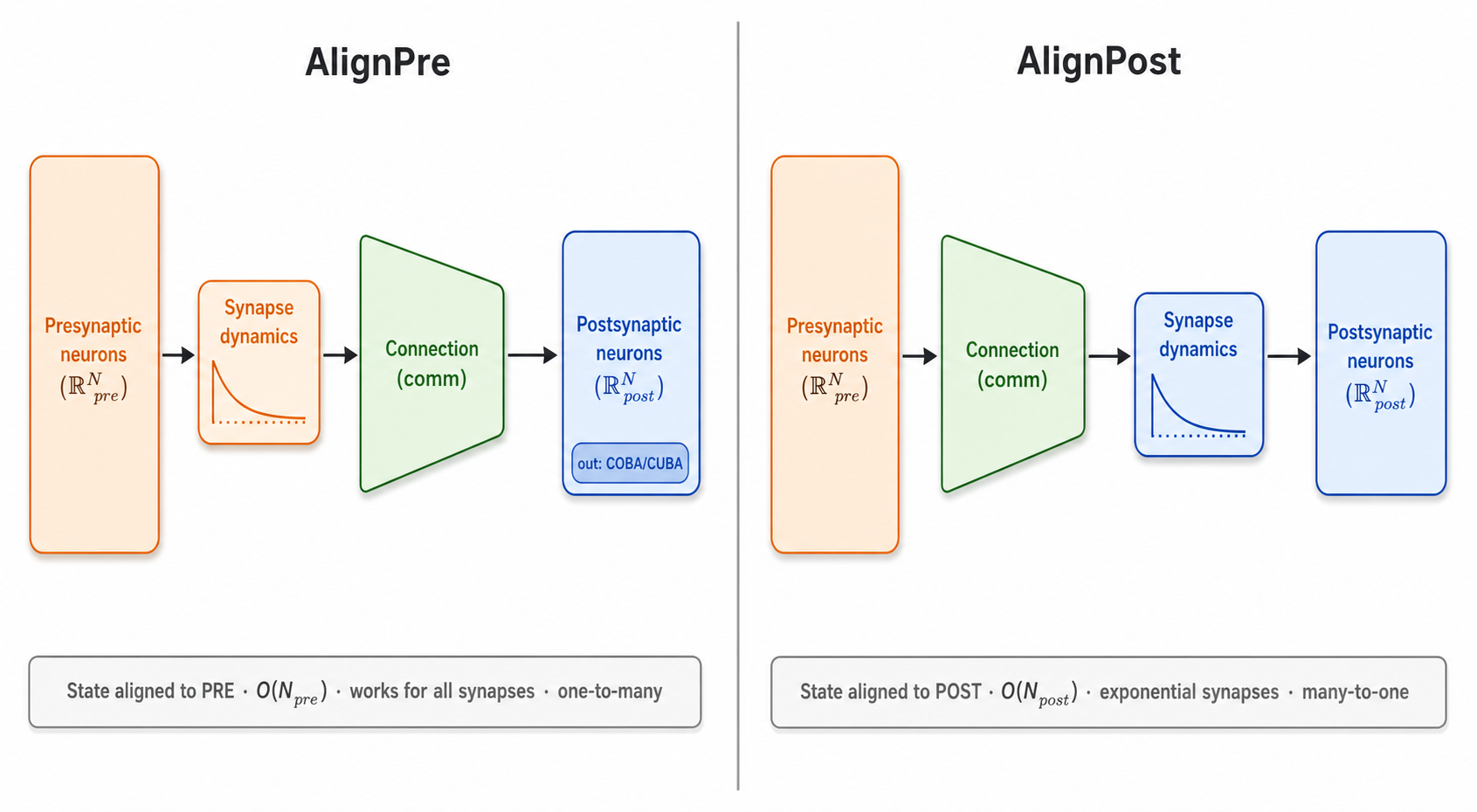
Fig. 2 AlignPre vs AlignPost. The synapse-dynamics block sits before the connection matrix on the left (state aligned to the presynaptic population, \(\mathcal{O}(N_\text{pre})\), works for all synapses, natural for one-to-many) and after it on the right (state aligned to the postsynaptic population, \(\mathcal{O}(N_\text{post})\), exponential-family synapses, natural for many-to-one). (Orange = presynaptic, blue = postsynaptic, green = connection matrix.)

4. AlignPost — state aligned to the postsynaptic neurons

Put the synapse dynamics after comm. Now the surviving state lives on the \(N_{\text{post}}\) postsynaptic neurons: memory is \(\mathcal{O}(N_{\text{post}})\), independent of how many presynaptic neurons or connections feed in.

Why is this exact? Recall the exponential synapse from Model anatomy: each arriving spike updates the postsynaptic conductance by \(g \leftarrow g + 1\), regardless of which presynaptic neuron emitted it. Spikes from many sources therefore superpose — their separate contributions sum linearly into one merged postsynaptic conductance. Tracking that single merged variable reproduces the full per-synapse dynamics with no approximation. The price of the trick is its precondition: it works only for synapse models with exponential (linear) dynamics.

AlignPost is the natural choice for many-to-one fan-in (the dominant pattern in recurrent networks) and is event-driven: only neurons that actually spiked contribute.

Worked example: the COBA excitatory–inhibitory network

The canonical balanced E–I network (Vogels & Abbott, 2005; Brette et al., 2007) wires 4000 neurons to themselves through two AlignPost projections — one excitatory (E = 0 mV), one inhibitory (E = -80 mV). Both use an exponential synapse, so AlignPost applies. Note syn and out are passed as describers (Expon.desc(...), COBA.desc(...)): the projection instantiates one shared postsynaptic synapse from the description.

import brainpy
import brainstate
import braintools
import brainunit as u
import matplotlib.pyplot as plt


class EINet(brainstate.nn.Module):
    def __init__(self):
        super().__init__()
        self.n_exc, self.n_inh = 3200, 800
        self.num = self.n_exc + self.n_inh
        # one postsynaptic population of 4000 LIF-with-refractory neurons
        self.N = brainpy.state.LIFRef(
            self.num,
            V_rest=-60. * u.mV, V_th=-50. * u.mV, V_reset=-60. * u.mV,
            tau=20. * u.ms, tau_ref=5. * u.ms,
            V_initializer=braintools.init.Normal(-55., 2., unit=u.mV),
        )
        # excitatory AlignPost projection: state aligned to the 4000 post neurons
        self.E = brainpy.state.AlignPostProj(
            comm=brainstate.nn.EventFixedProb(self.n_exc, self.num,
                                              conn_num=0.02, conn_weight=0.6 * u.mS),
            syn=brainpy.state.Expon.desc(self.num, tau=5. * u.ms),
            out=brainpy.state.COBA.desc(E=0. * u.mV),
            post=self.N,
        )
        # inhibitory AlignPost projection: shares the same post population
        self.I = brainpy.state.AlignPostProj(
            comm=brainstate.nn.EventFixedProb(self.n_inh, self.num,
                                              conn_num=0.02, conn_weight=6.7 * u.mS),
            syn=brainpy.state.Expon.desc(self.num, tau=10. * u.ms),
            out=brainpy.state.COBA.desc(E=-80. * u.mV),
            post=self.N,
        )

    def update(self, t, inp):
        with brainstate.environ.context(t=t):
            spk = self.N.get_spike() != 0.
            self.E(spk[:self.n_exc])   # excitatory neurons' spikes
            self.I(spk[self.n_exc:])   # inhibitory neurons' spikes
            self.N(inp)                # integrate synaptic + external current
            return self.N.get_spike()

An NVIDIA GPU may be present on this machine, but a CUDA-enabled jaxlib is not installed. Falling back to cpu.

net = EINet()
brainstate.nn.init_all_states(net)

with brainstate.environ.context(dt=0.1 * u.ms):
    times = u.math.arange(0. * u.ms, 1000. * u.ms, brainstate.environ.get_dt())
    spikes = brainstate.transform.for_loop(
        lambda t: net.update(t, 20. * u.mA), times,
        pbar=brainstate.transform.ProgressBar(10),
    )

# raster plot
t_idx, n_idx = u.math.where(spikes)
plt.figure(figsize=(10, 4))
plt.scatter(times[t_idx].to_decimal(u.ms), n_idx, s=0.5)
plt.xlabel('time (ms)'); plt.ylabel('neuron index')
plt.title('COBA E–I balanced network (two AlignPost projections)')
plt.tight_layout(); plt.show()

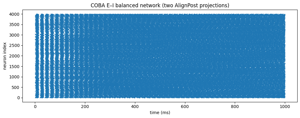
The synaptic state for each projection is a length-num (4000) vector — one entry per postsynaptic neuron — no matter how many presynaptic spikes arrive each step. That is the \(\mathcal{O}(N_{\text{post}})\) memory of AlignPost in practice.

5. AlignPre — state aligned to the presynaptic neurons

Put the synapse dynamics before comm. Now the surviving state lives on the \(N_{\text{pre}}\) presynaptic neurons: memory is \(\mathcal{O}(N_{\text{pre}})\).

Why exact here? With homogeneous synaptic parameters per presynaptic neuron, every synapse leaving a given source neuron is driven by the same spike train through the same dynamics — so they share one trace. Filter the spike train once per presynaptic neuron, then let comm distribute the result. Because the filtering happens before the (linear) connection matrix, the synapse model need not be linear: AlignPre works for all synapse models, including the voltage- and concentration-dependent ones — AMPA, GABAa, and BioNMDA (whose nonlinear kinetics rule out AlignPost).

AlignPre is the natural choice for one-to-many fan-out — one source population broadcasting to several targets, where the single per-source trace is reused for each.

The canonical AlignPre API

AlignPre is exposed as the function brainpy.state.align_pre_projection — there is intentionally no AlignPreProj class (AlignPost has both a class, AlignPostProj, and a function, align_post_projection). The function takes a spike generator, then the same four roles, with syn placed first in the pipeline so it filters in presynaptic space:

# A one-to-many fan-out with a nonlinear AMPA synapse -- AlignPost could not do this,
# because AMPA's kinetics are not a single linear exponential.
#
# Pattern (the canonical AlignPre call):
#
#   proj = brainpy.state.align_pre_projection(
#       pre,                                   # spike generator (the source population)
#       syn=brainpy.state.AMPA(n_pre),         # synapse dynamics in PRE space
#       comm=brainstate.nn.Linear(n_pre, n_post,
#                                 w_init=braintools.init.KaimingNormal(unit=u.mS),
#                                 b_init=None),
#       out=brainpy.state.COBA(E=0. * u.mV),   # conductance -> current
#       post=post,                             # postsynaptic population
#   )
#
# Per update: pre spikes -> syn filters them (one trace per presynaptic neuron)
#             -> comm distributes -> out -> post.
print('align_pre_projection is a function:',
      callable(brainpy.state.align_pre_projection))

align_pre_projection is a function: True

Seeing where the state lives

The defining property of AlignPre is that the synapse state is sized by the presynaptic population, not the postsynaptic one. The clearest way to show that is to assemble the pipeline from its lower-level pieces — a syn evolving in presynaptic space followed by a CurrentProj (the comm → out → post half that align_pre_projection wraps for you). Watch the shapes: syn.g has one entry per presynaptic neuron, while the postsynaptic voltage has one entry per target.

class FanOut(brainstate.nn.Module):
    def __init__(self, n_pre=400, n_post=100):
        super().__init__()
        self.pre = brainpy.state.LIF(
            n_pre, tau=20. * u.ms, V_rest=-60. * u.mV, V_th=-50. * u.mV,
            V_reset=-60. * u.mV,
            V_initializer=braintools.init.Normal(-55., 2., unit=u.mV))
        self.post = brainpy.state.LIF(
            n_post, tau=20. * u.ms, V_rest=-60. * u.mV, V_th=-50. * u.mV,
            V_reset=-60. * u.mV)
        # synapse in PRE space: its state vector is length n_pre
        self.syn = brainpy.state.Expon(
            n_pre, tau=5. * u.ms, g_initializer=braintools.init.Constant(0.))
        # comm -> out -> post (what align_pre_projection wraps internally)
        self.proj = brainpy.state.CurrentProj(
            comm=brainstate.nn.Linear(n_pre, n_post,
                                      w_init=braintools.init.KaimingNormal(unit=u.mS),
                                      b_init=None),
            out=brainpy.state.COBA(E=0. * u.mV),
            post=self.post,
        )

    def update(self, t, inp):
        with brainstate.environ.context(t=t):
            g_pre = self.syn(self.pre.get_spike())  # filter in PRE space
            self.proj(g_pre)                         # distribute to POST
            self.pre(inp)
            self.post(0. * u.mA)
            return self.post.get_spike()


net = FanOut()
brainstate.nn.init_all_states(net)
print('syn.g lives on PRE neurons  ->', net.syn.g.value.shape, '(== n_pre = 400)')
print('post.V lives on POST neurons ->', net.post.V.value.shape, '(== n_post = 100)')

with brainstate.environ.context(dt=0.1 * u.ms):
    times = u.math.arange(0. * u.ms, 100. * u.ms, brainstate.environ.get_dt())
    spk = brainstate.transform.for_loop(lambda t: net.update(t, 30. * u.mA), times)
print('post spike raster shape:', spk.shape)

syn.g lives on PRE neurons  -> (400,) (== n_pre = 400)
post.V lives on POST neurons -> (100,) (== n_post = 100)

post spike raster shape: (1000, 100)

The synapse vector is length 400 (the presynaptic count); the postsynaptic state is length 100. Broadcast that one source population to a second or third target and the same 400-entry trace is reused — that is the \(\mathcal{O}(N_{\text{pre}})\) payoff of AlignPre for one-to-many fan-out.

6. Exact, not approximate

It bears repeating, because it is the property that makes the whole design trustworthy rather than a heuristic:

These projections are not approximations. They accurately compute the same dynamics as the original projections while providing new benefits. — Wang et al., ICLR 2024.

Each alignment is exact under its stated condition:

• AlignPre requires homogeneous synaptic parameters per presynaptic neuron, so that all synapses from one source share a single trace. As the paper puts it: “with homogeneous synaptic parameters, the spike train coming from the same presynaptic neuron will lead to the same synaptic dynamics … all synapses originating from the same presynaptic neuron can share a single dynamical variable … AlignPre … is suitable for all types of synapse models.”

• AlignPost requires linear (exponential) synaptic dynamics, so that contributions superpose. Again from the paper: “the applicability of AlignPost is limited to synapse models that exhibit exponential dynamics … the conductance g of a post-synaptic neuron is updated according to \(g \leftarrow g + 1\) whenever a spike arrives and regardless of which presynaptic neuron emitted this spike.”

When its condition holds, the reduction changes the memory footprint and nothing else.

7. Automatic merging

Because synaptic state is keyed by a neuron dimension (plus the synapse/output description), projections that target the same place with the same kinetics can share a single synapse instance automatically:

• AlignPost — multiple projections into the same post population with the same syn/out descriptor share one postsynaptic synapse; their inputs sum into the merged conductance.

• AlignPre — projections from the same pre population (with the same delay) share one presynaptic synapse.

This is the additive-input convention from Model anatomy paying off: convergent pathways merge with no extra memory, and you express them simply by pointing several projections at the same population.

8. Choosing between them

Reach for AlignPost when synapses are exponential-family and the wiring fans in (many sources, one target) — the common recurrent-network case. Reach for AlignPre when the synapse is nonlinear, or when one source fans out to many targets. Both are exact; the choice is about which dimension is smaller and which condition your synapse satisfies.

Table 1 When to use AlignPre vs AlignPost

Want	Synapse type	Connectivity	Use	State
Event-driven fan-in	exponential-family (Expon, DualExpon)	many → one	AlignPost (AlignPostProj / align_post_projection)	\(\mathcal{O}(N_\text{post})\)
Nonlinear kinetics	AMPA, BioNMDA, GABAa	any	AlignPre (align_pre_projection)	\(\mathcal{O}(N_\text{pre})\)
One source → many targets	any	one → many	AlignPre (align_pre_projection)	\(\mathcal{O}(N_\text{pre})\)
Direct current / no synapse dynamics	—	any	CurrentProj / DeltaProj	—

Table 2 The three memory regimes

Scheme	State lives on	State memory	Applies to	Best for
Naïve per-synapse	each synapse	\(\mathcal{O}(p \cdot N_\text{pre} \cdot N_\text{post})\)	any	(wasteful)
AlignPre	presynaptic neurons	\(\mathcal{O}(N_\text{pre})\)	all synapse models	one-to-many
AlignPost	postsynaptic neurons	\(\mathcal{O}(N_\text{post})\)	exponential-family only	many-to-one

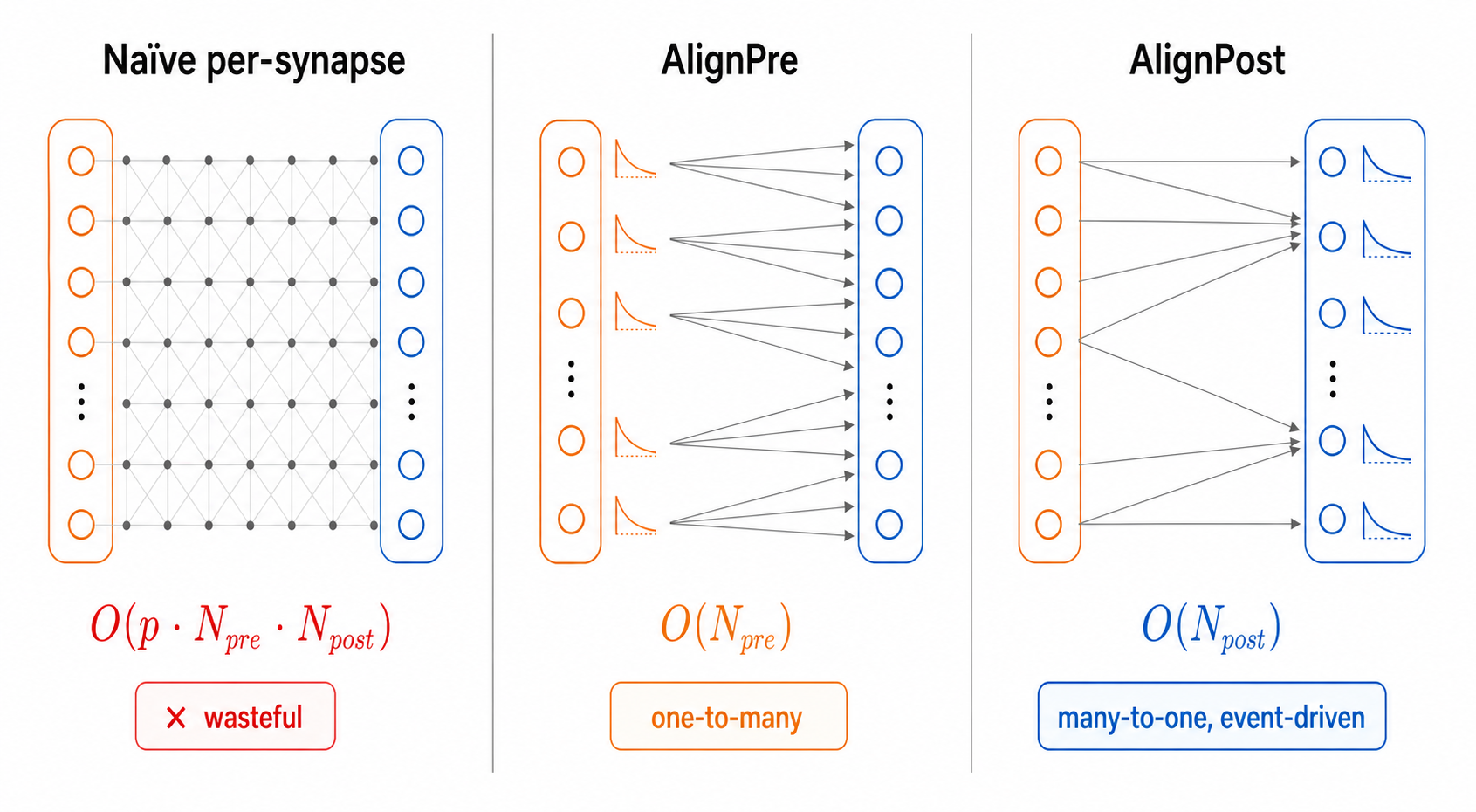
Fig. 3 Three memory regimes. Naive per-synapse state scales with the number of connections; AlignPre collapses it onto the presynaptic neurons (\(\mathcal{O}(N_\text{pre})\)) and AlignPost onto the postsynaptic neurons (\(\mathcal{O}(N_\text{post})\)) — both exactly.

9. The bridge to learning

Here is why this chapter is the keystone of the whole framework, not just a memory optimization.

Aligning synaptic state to a neuron dimension instead of a weight dimension does more than shrink the forward pass. It is also what makes gradient-based and online learning tractable. Backpropagation-through-time differentiates the very for_loop you used above, and neuron-aligned state keeps the activations it must remember small (see Differentiability). More dramatically, in real-time recurrent learning (RTRL) the same superposition that makes AlignPost’s forward pass exact is reused on the backward pass: the eligibility traces and Jacobians that would otherwise scale cubically/quadratically with the number of hidden units collapse to linear memory. That is the result of Wang et al. (2026, Nature Communications), and it is what puts whole-brain-scale online learning within reach.

In one sentence: the alignment that makes simulation memory-efficient is the alignment that makes learning memory-efficient. The two worlds — brain simulation and brain-inspired computing — meet exactly here.

Continue to Online learning for the linear-memory story.

10. API pointers

• AlignPost — class brainpy.state.AlignPostProj and function brainpy.state.align_post_projection (syn/out as .desc(...) describers).

• AlignPre — function brainpy.state.align_pre_projection (no class).

• Direct injection — brainpy.state.CurrentProj (continuous current, no synapse) and brainpy.state.DeltaProj (instantaneous delta input).

• Gap junctions — brainpy.state.SymmetryGapJunction / brainpy.state.AsymmetryGapJunction for electrical coupling.

• Short-term plasticity — pass stp=brainpy.state.STP(...) (or STD) to align_pre_projection / align_post_projection.

See API Reference for full signatures.

References

• Wang, C., Zhang, T., He, S., Gu, H., Li, S., Wu, S. (2024). A differentiable brain simulator bridging brain simulation and brain-inspired computing. ICLR 2024. https://openreview.net/forum?id=AU2gS9ut61 (arXiv:2311.05106). — introduces AlignPre / AlignPost.

• Vogels, T. P. & Abbott, L. F. (2005). Signal propagation and logic gating in networks of integrate-and-fire neurons. J. Neurosci. 25(46), 10786–95. — the balanced E–I network reproduced above.

See also

• Model anatomy — the comm / syn / out / post pieces and the g ← g + 1 increment this design exploits.

• Differentiability — backpropagation-through-time over the same models.

• Online learning — linear-memory RTRL, the learning-side payoff.

• BrainPy-style Modeling — projections applied in tutorials and how-to guides.