
Populations and devices#
What you’ll learn / who it’s for (simulation). Scale from one neuron to populations: create groups of NEST-compatible neurons, combine and slice them with NodeView algebra, attach stimulation and recording devices, and read population spikes back as a raster and a firing rate.
Mirrors PyNEST Part 2 in the brainpy.state idiom.
import jax
jax.config.update('jax_enable_x64', True)
import brainstate
brainstate.environ.set(precision=64)

import numpy as np
import brainunit as u
import braintools
import matplotlib.pyplot as plt
from brainpy import state as bp
An NVIDIA GPU may be present on this machine, but a CUDA-enabled jaxlib is not installed. Falling back to cpu.
Creating a population#
sim.create(model, N, ...) makes a population of N neurons and returns a NodeView. Parameters use NEST’s names and units; for a large set, pass a params=dict(...) mapping. Here we build an excitatory and an inhibitory population of current-based IAF neurons.
npar = dict(C_m=250. * u.pF, tau_m=20. * u.ms, t_ref=2. * u.ms,
            E_L=0. * u.mV, V_reset=0. * u.mV, V_th=20. * u.mV,
            V_initializer=braintools.init.Constant(0. * u.mV))

sim = bp.Simulator(dt=0.1 * u.ms)
ne = sim.create(bp.iaf_psc_alpha, 80, params=npar)    # excitatory
ni = sim.create(bp.iaf_psc_alpha, 20, params=npar)    # inhibitory
print('ne:', ne, '\nni:', ni)
ne: <brainpy.state.NodeView object at 0x7f57b582fe00>
ni: <brainpy.state.NodeView object at 0x7f57b59cf750>
NodeView algebra: combine and slice#
Two operators let a single connect target a combined or partial population:
concatenate —
ne + niis the whole network (E then I),slice —
ne[:10]is the first 10 excitatory neurons.
We drive both populations with a shared Poisson background (all_to_all) and record a sub-sample of each.
noise = sim.create(bp.poisson_generator, rate=8000. * u.Hz, rng_seed=0)
esr = sim.create(bp.spike_recorder)
isr = sim.create(bp.spike_recorder)

sim.connect(noise, ne + ni, weight=10. * u.pA, delay=1.5 * u.ms, rule=bp.all_to_all)
sim.connect(ne[:10], esr)            # record the first 10 excitatory
sim.connect(ni[:10], isr)            # record the first 10 inhibitory

res = sim.simulate(500. * u.ms)
Reading population output: rate and raster#
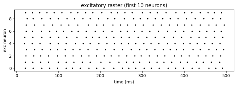
res.rate(view) gives the mean firing rate (Hz) and res.spikes(view) gives the per-step spike matrix (T, N) we can scatter into a raster.
print(f'exc rate: {res.rate(esr):.2f} spks/s')
print(f'inh rate: {res.rate(isr):.2f} spks/s')

spk = np.asarray(res.spikes(esr))           # (T, 10)
ts, ids = np.nonzero(spk > 0)
t_ms = np.asarray(u.get_mantissa(res.times / u.ms))
plt.figure(figsize=(8, 3))
plt.scatter(t_ms[ts], ids, s=4, color='k')
plt.xlabel('time (ms)'); plt.ylabel('exc neuron')
plt.title('excitatory raster (first 10 neurons)')
plt.tight_layout()
exc rate: 51.20 spks/s
inh rate: 50.20 spks/s
See also#
One neuron — the single-neuron starting point.
Connect a network — recurrent wiring rules.
Connectivity —
NodeViewalgebra and rules.Devices — the full device catalog.