
One neuron#
What you’ll learn / who it’s for (simulation). The NEST-compatible first step: create a single iaf_psc_alpha, drive it with a constant current and then with Poisson noise, and record its membrane potential and spikes — all through the brainpy.state Simulator API, which mirrors NEST’s vocabulary (create / connect / simulate).
This is the brainpy.state idiom, not a copy of PyNEST: we build with physical units (brainunit) and let the Simulator lower the time loop. For the biophysics of iaf_psc_alpha, follow the link out to the NEST documentation.
import jax
jax.config.update('jax_enable_x64', True)
import brainstate
brainstate.environ.set(precision=64)

import numpy as np
import brainunit as u
import matplotlib.pyplot as plt
from brainpy import state as bp
An NVIDIA GPU may be present on this machine, but a CUDA-enabled jaxlib is not installed. Falling back to cpu.
A single neuron driven by a constant current#
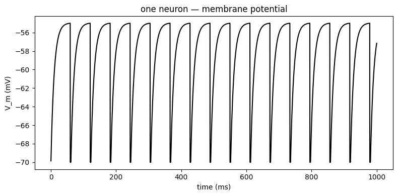
We create one iaf_psc_alpha with a constant external current I_e = 376 pA and attach a voltmeter. As in NEST, the voltmeter is connected in the reversed direction — connect(voltmeter, neuron) — because it observes the neuron rather than receiving events from it. With I_e = 376 pA the steady state sits just above threshold, so the neuron charges, fires, and repeats.
sim = bp.Simulator(dt=0.1 * u.ms)
neuron = sim.create(bp.iaf_psc_alpha, 1, I_e=376. * u.pA)
vm = sim.create(bp.voltmeter)
sim.connect(vm, neuron)              # reversed: the voltmeter observes the neuron

res = sim.simulate(1000. * u.ms)
sim.simulate(T) runs the whole simulation (it lowers the time loop internally — there is no bare Python loop over steps). We read the recorded trace back from the result with res.trace(vm, 'V_m') and the time axis with res.times.
t = np.asarray(u.get_mantissa(res.times / u.ms))
v = np.asarray(u.get_mantissa(res.trace(vm, 'V_m') / u.mV)).reshape(-1)
n_spikes = int((np.diff(v) < -10.0).sum())   # threshold resets show as big drops
print(f'V_m: start {v[0]:.2f} mV, max {v.max():.2f} mV, {n_spikes} spikes in 1000 ms')

plt.figure(figsize=(8, 4))
plt.plot(t, v, color='k')
plt.xlabel('time (ms)'); plt.ylabel('V_m (mV)')
plt.title('one neuron — membrane potential')
plt.tight_layout()
V_m: start -69.85 mV, max -55.00 mV, 16 spikes in 1000 ms
Driving the neuron with Poisson noise#
Now replace the DC drive with a 2-channel poisson_generator — an excitatory channel and an inhibitory channel — with signed per-channel weights [1.2, -1.0] pA. The generator fans out one independent train per channel, and the per-channel weight vector applies one signed weight each, so the neuron integrates 1.2 · train_ex − 1.0 · train_in. A passive spike_recorder lets us read the firing rate back.
sim = bp.Simulator(dt=0.1 * u.ms)
neuron = sim.create(bp.iaf_psc_alpha, 1)
noise = sim.create(bp.poisson_generator, 2, rate=[80000., 15000.] * u.Hz, rng_seed=0)
vm = sim.create(bp.voltmeter)
sr = sim.create(bp.spike_recorder)

sim.connect(noise, neuron, weight=[1.2, -1.0] * u.pA, delay=1.0 * u.ms)
sim.connect(vm, neuron)              # reversed analog tap
sim.connect(neuron, sr)             # the spike recorder taps the neuron

res = sim.simulate(1000. * u.ms)
v = np.asarray(u.get_mantissa(res.trace(vm, 'V_m') / u.mV)).reshape(-1)
print(f'V_m: mean {v.mean():.2f} mV, std {v.std():.2f} mV')
print(f'firing rate: {res.rate(sr):.2f} spks/s')
V_m: mean -61.25 mV, std 4.96 mV
firing rate: 47.00 spks/s
See also#
Populations & devices — scale up to populations.
Model directory — the neuron families.
Devices — generators, recorders, and detectors.
The State paradigm — why
brainpy.statemakes state explicit and how the loop is lowered.