
Differentiability#
What you’ll learn / who it’s for (training). The simulator → trainable half of
the bridge. Spiking models in brainpy.state are differentiable: a surrogate
gradient replaces the non-differentiable spike threshold, and
backpropagation-through-time runs straight over the transform loops you already
use to simulate. You’ll plug in a surrogate, train a tiny SNN end to end, and learn
when to switch to checkpointed loops for long rollouts.
1. Why spikes need surrogate gradients#
A spike is a step function of the membrane potential: it is \(0\) below threshold and \(1\) at threshold. Its derivative is zero almost everywhere and undefined at the threshold itself — useless for gradient descent, which would see no signal to follow.
The surrogate gradient trick keeps the hard spike on the forward pass (so the
dynamics are exactly the spiking dynamics) but substitutes a smooth, well-behaved
function on the backward pass — a narrow bump centered at threshold. You select one
by passing spk_fun= to any neuron; braintools.surrogate provides the
standard family.
import brainpy
import brainstate
import braintools
import brainunit as u
import jax.numpy as jnp
import matplotlib.pyplot as plt

# A LIF neuron whose backward pass uses a ReLU-shaped surrogate gradient.
neuron = brainpy.state.LIF(
    100,
    tau=20. * u.ms, V_rest=0. * u.mV, V_reset=0. * u.mV, V_th=1. * u.mV,
    spk_fun=braintools.surrogate.ReluGrad(),
)
print('surrogate:', neuron.spk_fun)
An NVIDIA GPU may be present on this machine, but a CUDA-enabled jaxlib is not installed. Falling back to cpu.
surrogate: ReluGrad(alpha=0.3, width=1.0)
Other choices include braintools.surrogate.SigmoidGrad(), GaussianGrad(),
and SuperSpike() — they differ only in the shape of the backward-pass bump.
ReluGrad is a robust default.
2. Backprop through time with transform#
Two facts make training work without any special machinery:
The
brainstate.transformloops —for_loopandscan— are differentiable. Wrapping a simulation infor_loopand askingbrainstate.transform.gradfor gradients gives you backpropagation-through-time (BPTT) over the unrolled trajectory.brainstate.transform.graddifferentiates with respect to exactly theParamStatevariables you select (net.states(brainstate.ParamState)), leaving dynamical state alone.
The recipe is therefore: build the network, define a loss that runs it with
for_loop and reduces over time, then take its gradient with respect to the
parameters — all inside a single jit-compiled train step.
Memory warning. Plain BPTT stores the activations of every unrolled step for the backward pass, so peak memory grows with rollout length. For long rollouts use
brainstate.transform.checkpointed_for_loop/checkpointed_scan(§4).
3. A small runnable trainable example#
A three-layer SNN — input → recurrent LIF → readout — trained to classify random
spike patterns. This is the canonical training pattern: a loss_fn that simulates
with for_loop and averages the readout over time, a jit-compiled
train_step that resets state, takes gradients, and steps the optimizer, and a
plain-Python outer epoch loop (which is allowed — the rule against bare loops is
about time-stepping the model, not about optimization).
with brainstate.environ.context(dt=1.0 * u.ms):
class SNN(brainstate.nn.Module):
def __init__(self, n_in, n_rec, n_out):
super().__init__()
# input -> recurrent: a trainable Linear (weights in mA) feeding an
# exponential synapse
self.i2r = brainstate.nn.Sequential(
brainstate.nn.Linear(
n_in, n_rec,
w_init=braintools.init.KaimingNormal(unit=u.mA),
b_init=braintools.init.ZeroInit(unit=u.mA)),
brainpy.state.Expon(n_rec, tau=5. * u.ms,
g_initializer=braintools.init.Constant(0. * u.mA)),
)
# recurrent LIF with a surrogate gradient -> this is what makes it trainable
self.r = brainpy.state.LIF(
n_rec, tau=20. * u.ms, V_reset=0. * u.mV, V_rest=0. * u.mV,
V_th=1. * u.mV, spk_fun=braintools.surrogate.ReluGrad())
# recurrent -> output readout
self.r2o = brainstate.nn.Linear(n_rec, n_out,
w_init=braintools.init.KaimingNormal())
self.o = brainpy.state.Expon(n_out, tau=10. * u.ms,
g_initializer=braintools.init.Constant(0.))
def update(self, spike):
return self.o(self.r2o(self.r(self.i2r(spike))))
# tiny synthetic dataset: random Poisson-like input spikes, binary labels
n_in = 100
net = SNN(n_in=n_in, n_rec=4, n_out=2)
num_step, num_sample = 100, 128
freq = 5 * u.Hz
x_data = brainstate.random.rand(num_step, num_sample, n_in) \
< freq * brainstate.environ.get_dt()
y_data = u.math.asarray(brainstate.random.rand(num_sample) < 0.5, dtype=int)
# optimizer registered on the trainable parameters only
optimizer = braintools.optim.Adam(lr=3e-3)
optimizer.register_trainable_weights(net.states(brainstate.ParamState))
def loss_fn():
# for_loop over time -> BPTT-able trajectory of readouts [T, B, C]
preds = brainstate.transform.for_loop(net.update, x_data)
preds = u.math.mean(preds, axis=0) # average readout over time -> [B, C]
return braintools.metric.softmax_cross_entropy_with_integer_labels(
preds, y_data).mean()
@brainstate.transform.jit
def train_step():
brainstate.nn.init_all_states(net, batch_size=num_sample) # reset each step
grads, loss = brainstate.transform.grad(
loss_fn, net.states(brainstate.ParamState), return_value=True)()
optimizer.update(grads)
return loss
# outer optimization loop in plain Python -- this is fine
losses = []
for epoch in range(1, 201):
losses.append(float(train_step()))
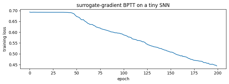
plt.figure(figsize=(8, 3))
plt.plot(losses)
plt.xlabel('epoch'); plt.ylabel('training loss')
plt.title('surrogate-gradient BPTT on a tiny SNN')
plt.tight_layout(); plt.show()
The full version of this example (with a Fashion-MNIST-scale dataset and accuracy reporting) is in the training how-to track — see How to use surrogate gradients.
4. Long rollouts: checkpoint to bound memory#
Because BPTT stores every step’s activations, a long simulation can exhaust memory on the backward pass. The checkpointed loop variants trade compute for memory: they keep only a sparse set of checkpoints on the forward pass and recompute the intervening activations during backprop.
Swap the loop and tune the base parameter (larger base → fewer checkpoints →
less memory, more recomputation); the semantics are otherwise identical to
for_loop / scan:
preds = brainstate.transform.checkpointed_for_loop(net.update, x_data)
# or, with an explicit carry:
# carry, ys = brainstate.transform.checkpointed_scan(step, carry0, xs)
Reach for these only when reverse-mode gradients through a long rollout would
otherwise run out of memory — for ordinary-length rollouts, plain for_loop /
scan is simpler and faster. The dedicated how-to walks through the trade-off:
How to train through long rollouts without exhausting memory.
Recap#
A spike’s gradient is unusable; a surrogate (
spk_fun=...) supplies a smooth backward pass while the forward pass stays exactly spiking.transform.for_loop/scanare differentiable, so wrapping a simulation in them and callingtransform.gradis backpropagation-through-time.Select trainable variables with
net.states(brainstate.ParamState); reset state each step withinit_all_states.For long rollouts, switch to
checkpointed_for_loop/checkpointed_scanto bound memory.
See also#
AlignPre / AlignPost — the keystone — why neuron-aligned state keeps BPTT activations small, and the keystone the next page builds on.
Online learning — the trainable → scalable half: linear-memory RTRL.
The state paradigm — the
transformprimitives used here.How to use surrogate gradients — the full training how-to.