
Tutorial 1 · Your first neuron#
What you’ll learn. How to instantiate a single spiking neuron from the BrainPy-style library, inject an input current, run it forward in time, and inspect its membrane potential and spike train.
Who it’s for. Everyone — this is the entry point. No prior knowledge of the API is assumed. (Audience: simulation and training.)
We use the leaky integrate-and-fire neuron with a refractory period,
brainpy.state.LIFRef. A neuron is a state-based Module: it owns its dynamical
variables (here the membrane potential V) as explicit State objects, and you
advance it one time step per call. To run it over many steps we never write a
bare Python for loop — we hand the per-step function to
brainstate.transform.for_loop, which compiles the whole rollout into a single
XLA program and stacks the outputs for us.
import brainpy
import brainstate
import braintools
import brainunit as u
import matplotlib.pyplot as plt
An NVIDIA GPU may be present on this machine, but a CUDA-enabled jaxlib is not installed. Falling back to cpu.
Create the neuron#
All quantities carry physical units (millivolts, milliseconds, …) via
brainunit. The constructor takes the population size first — here a single
neuron — followed by the membrane parameters.
with brainstate.environ.context(dt=0.1 * u.ms):
    neuron = brainpy.state.LIFRef(
        1,                     # one neuron
        R=1. * u.ohm,          # membrane resistance
        tau=20. * u.ms,        # membrane time constant
        V_rest=-60. * u.mV,    # resting potential
        V_th=-50. * u.mV,      # spike threshold
        V_reset=-60. * u.mV,   # reset after a spike
        tau_ref=5. * u.ms,     # refractory period
    )
    # Allocate the neuron's state variables (V, last_spike_time).
    brainstate.nn.init_all_states(neuron)

print(neuron)
LIFRef(
  in_size=(1,),
  out_size=(1,),
  spk_reset=soft,
  spk_fun=ReluGrad(alpha=0.3, width=1.0),
  R=Quantity(1., "ohm"),
  tau=Quantity(20., "ms"),
  tau_ref=Quantity(5., "ms"),
  V_th=Quantity(-50., "mV"),
  V_rest=Quantity(-60., "mV"),
  V_reset=Quantity(-60., "mV"),
  V_initializer=Constant(value=0. mV),
  V=HiddenState(
    value=Quantity(~float32[1], "mV")
  ),
  last_spike_time=ShortTermState(
    value=Quantity(~float32[1], "ms")
  )
)
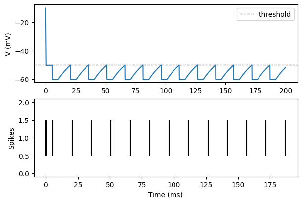
Drive it with a constant current#
We define a single-step function that (1) opens an environ.context so the
model knows the current time t, (2) advances the neuron by one step with an
injected current, and (3) returns what we want to record. Then for_loop
repeats it across an array of time points.
get_spike() returns the spike output of the neuron for the current step.
with brainstate.environ.context(dt=0.1 * u.ms):
    times = u.math.arange(0. * u.ms, 200. * u.ms, brainstate.environ.get_dt())

    def step(t):
        with brainstate.environ.context(t=t):
            neuron(25. * u.mA)                 # inject a supra-threshold current
            return neuron.V.value, neuron.get_spike()

    vs, spikes = brainstate.transform.for_loop(step, times)

print('membrane trace shape:', vs.shape)
print('total spikes:', float(u.math.sum(spikes)))
membrane trace shape: (2000, 1)
total spikes: 17.0
Plot the membrane potential and spikes#
vs is a brainunit quantity; convert it to millivolts for plotting. The spike
times are simply the time points where the spike output is non-zero.
t_ms = times.to_decimal(u.ms)
v_mV = vs.to_decimal(u.mV)[:, 0]

fig, gs = braintools.visualize.get_figure(2, 1, 2.0, 6.0)

ax = fig.add_subplot(gs[0, 0])
ax.plot(t_ms, v_mV)
ax.axhline(-50., ls='--', color='gray', lw=1, label='threshold')
ax.set_ylabel('V (mV)')
ax.legend(loc='upper right')

ax = fig.add_subplot(gs[1, 0])
spk_idx, _ = u.math.where(spikes)
ax.eventplot(t_ms[spk_idx], colors='k')
ax.set_xlabel('Time (ms)')
ax.set_ylabel('Spikes')
plt.show()
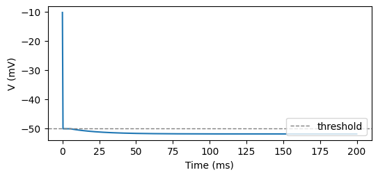
Sub-threshold vs. supra-threshold input#
A weaker current never reaches threshold, so the neuron charges toward a steady state and never fires. Re-initialize the state and drive it more gently to see the difference.
with brainstate.environ.context(dt=0.1 * u.ms):
    brainstate.nn.init_all_states(neuron)   # reset V back to rest

    def step_weak(t):
        with brainstate.environ.context(t=t):
            neuron(8. * u.mA)                 # sub-threshold drive
            return neuron.V.value

    vs_weak = brainstate.transform.for_loop(step_weak, times)

plt.figure(figsize=(6, 2.5))
plt.plot(t_ms, vs_weak.to_decimal(u.mV)[:, 0])
plt.axhline(-50., ls='--', color='gray', lw=1, label='threshold')
plt.xlabel('Time (ms)')
plt.ylabel('V (mV)')
plt.legend(loc='lower right')
plt.show()
See also#
Tutorial 2 · Synapses and projections — connect two populations of these neurons.
The state paradigm — why models hold explicit
Stateand why we drive them withtransformloops instead of Python loops.Physical units — the
brainunitquantities used throughout.Model anatomy — the
Dynamics → Neuronhierarchy and the current-input contract.How to choose a neuron model — pick a different neuron model.