
Tutorial 4 · Train a spiking network#
What you’ll learn. How to turn a spiking network into a trainable model:
plug a surrogate gradient into the spiking nonlinearity, run the network over
time with for_loop, and take gradient-descent steps with an optimizer.
Who it’s for. Readers who have built a network (tutorials 1–3) and now want to train it. (Audience: training / brain-inspired computing.)
The spike threshold is a step function, so its derivative is zero almost
everywhere — vanilla backprop would see no gradient. The fix is a surrogate
gradient: the forward pass still emits hard spikes, but the backward pass uses
a smooth surrogate derivative. In brainpy.state you simply pass a
braintools.surrogate function as spk_fun=. The rest is ordinary deep-learning
machinery, with one twist: the per-step for_loop is differentiable, so
gradients flow backward through time (BPTT) automatically.
To keep this notebook self-contained we train on a small synthetic classification task rather than downloading a dataset. The same recipe scales to MNIST / Fashion-MNIST — see the gallery scripts.
import brainpy
import brainstate
import braintools
import brainunit as u
import matplotlib.pyplot as plt
import numpy as np
An NVIDIA GPU may be present on this machine, but a CUDA-enabled jaxlib is not installed. Falling back to cpu.
A feed-forward spiking classifier#
Three stages: an input→recurrent synapse (a linear layer feeding an exponential
synapse), a recurrent LIF layer whose spk_fun is the surrogate, and a
readout→output synapse. Calling the network once advances every stage by one
time step.
class SNN(brainstate.nn.Module):
    def __init__(self, n_in, n_rec, n_out):
        super().__init__()
        self.i2r = brainstate.nn.Sequential(
            brainstate.nn.Linear(
                n_in, n_rec,
                w_init=braintools.init.KaimingNormal(unit=u.mA),
                b_init=braintools.init.ZeroInit(unit=u.mA)),
            brainpy.state.Expon(
                n_rec, tau=5. * u.ms,
                g_initializer=braintools.init.Constant(0. * u.mA)),
        )
        # the surrogate gradient lives here, on the spiking layer
        self.r = brainpy.state.LIF(
            n_rec, tau=20. * u.ms,
            V_rest=0. * u.mV, V_reset=0. * u.mV, V_th=1. * u.mV,
            spk_fun=braintools.surrogate.ReluGrad(),
        )
        self.r2o = brainstate.nn.Linear(
            n_rec, n_out, w_init=braintools.init.KaimingNormal())
        self.o = brainpy.state.Expon(
            n_out, tau=10. * u.ms,
            g_initializer=braintools.init.Constant(0.))

    def update(self, spike):
        return self.o(self.r2o(self.r(self.i2r(spike))))
A synthetic dataset#
Each sample is a [T, B, n_in] tensor of Poisson input spikes; the label is a
random binary class. The network’s job is to map the spike pattern to its class.
with brainstate.environ.context(dt=1.0 * u.ms):
    n_in, n_rec, n_out = 100, 4, 2
    num_step, num_sample = 200, 256
    freq = 5. * u.Hz

    x_data = brainstate.random.rand(num_step, num_sample, n_in) < freq * brainstate.environ.get_dt()
    x_data = x_data.astype(float)
    y_data = u.math.asarray(brainstate.random.rand(num_sample) < 0.5, dtype=int)

print('inputs:', x_data.shape, '  labels:', y_data.shape)
inputs: (200, 256, 100) labels: (256,)
Loss, optimizer, and a compiled train step#
The loss runs the network over all time steps with for_loop, averages the
output over time, and applies a cross-entropy. The train step is JIT-compiled and
takes one gradient step; the outer epoch loop is an ordinary Python loop —
that is fine, because each iteration calls the compiled step. (The rule is never
to time-step a model with a bare Python loop, which we don’t: time-stepping
goes through for_loop.)
with brainstate.environ.context(dt=1.0 * u.ms):
net = SNN(n_in, n_rec, n_out)
optimizer = braintools.optim.Adam(lr=3e-3)
optimizer.register_trainable_weights(net.states(brainstate.ParamState))
def loss_fn():
preds = brainstate.transform.for_loop(net.update, x_data) # [T, B, C]
preds = u.math.mean(preds, axis=0) # [B, C]
return braintools.metric.softmax_cross_entropy_with_integer_labels(
preds, y_data).mean()
@brainstate.transform.jit
def train_step():
brainstate.nn.init_all_states(net, batch_size=num_sample)
grads, loss = brainstate.transform.grad(
loss_fn, net.states(brainstate.ParamState), return_value=True)()
optimizer.update(grads)
return loss
losses = []
for epoch in range(1, 201): # outer optimization loop — OK
losses.append(float(train_step()))
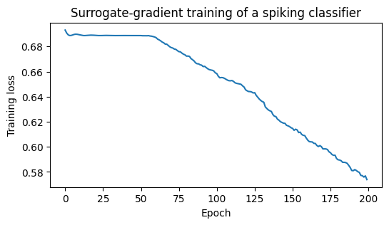
print('first loss: %.4f last loss: %.4f' % (losses[0], losses[-1]))
first loss: 0.6931 last loss: 0.5738
The training curve#
plt.figure(figsize=(6, 3))
plt.plot(np.asarray(losses))
plt.xlabel('Epoch')
plt.ylabel('Training loss')
plt.title('Surrogate-gradient training of a spiking classifier')
plt.show()
See also#
Differentiability — surrogate gradients and BPTT through the transform loops, in depth.
How to use surrogate gradients — compare different surrogate functions.
How to add a trainable readout — use a
LeakyRateReadouthead instead of averaging.How to train through long rollouts without exhausting memory — bound memory for long rollouts with
checkpointed_for_loop.