
Model anatomy#
What you’ll learn / who it’s for (simulation and training). The shared
Dynamics contract behind every neuron and synapse — the state variables they
own, the update() step, the get_spike() output, and how a neuron receives
current. This contract is exactly what projections rely on, so it sets up the
keystone chapter that follows.
One contract: Dynamics#
brainpy.state models form a small, deliberate hierarchy:
brainstate.nn.Module
└── Dynamics            (anything that evolves in time)
    ├── Neuron          (a population that integrates current and emits spikes)
    └── Synapse         (temporal filtering of a spike train)
Every Dynamics honors the same four-part contract:
Declare state in
__init__(e.g. membrane potentialV, conductanceg).Allocate it via
init_all_states(which calls each object’sinit_state).Advance one step with
update(...)— called for you when you invoke the module.Expose outputs — neurons add
get_spike().
Because the contract is uniform, components compose: a Synapse filters spikes
into a current, and a Neuron integrates that current — and a projection
(next chapter) snaps the two together across populations.
import brainpy
import brainstate
import braintools
import brainunit as u
import jax.numpy as jnp
import matplotlib.pyplot as plt
An NVIDIA GPU may be present on this machine, but a CUDA-enabled jaxlib is not installed. Falling back to cpu.
Neurons: integrate current, emit spikes#
A neuron population owns a membrane potential V (a state) and a set of unitful
parameters (tau, V_th, V_reset, V_rest, R). Calling the neuron
with an input current advances V one dt and, when V crosses threshold,
emits a spike and resets.
neuron = brainpy.state.LIFRef(
    100,
    V_rest=-65. * u.mV, V_th=-50. * u.mV, V_reset=-65. * u.mV,
    tau=10. * u.ms, tau_ref=2. * u.ms,
    V_initializer=braintools.init.Normal(-65., 2., unit=u.mV),
)
brainstate.nn.init_all_states(neuron)

print('state variable V:', neuron.V.value.shape, neuron.V.value.dtype)
state variable V: (100,) float32
get_spike(): the spike output#
A neuron’s spike output is read with get_spike(). During training it is a
surrogate — a smooth, differentiable stand-in for the hard threshold (see
Differentiability) — but its role in wiring is always the same: it
is the signal a projection transmits to downstream populations.
def step(t):
    with brainstate.environ.context(t=t):
        neuron(jnp.ones(100) * 30. * u.mA)   # drive every neuron
        return neuron.V.value, neuron.get_spike()

with brainstate.environ.context(dt=0.1 * u.ms):
    times = u.math.arange(0. * u.ms, 100. * u.ms, brainstate.environ.get_dt())
    vs, spikes = brainstate.transform.for_loop(step, times)

print('voltage trace:', vs.shape)      # (time, neurons)
print('spike trace:  ', spikes.shape)  # (time, neurons)
print('total spikes: ', int(u.math.sum(spikes)))
voltage trace: (1000, 100)
spike trace:   (1000, 100)
total spikes: 1100
How a neuron receives current#
Synaptic input does not overwrite a neuron’s drive — it accumulates into it.
Internally a neuron sums all current contributions delivered during a step before
integrating V. From your side this means you simply call the neuron with any
direct input, and projections add their synaptic current on top:
self.proj(pre_spikes)   # projection deposits synaptic current into `post`
self.post(external)     # neuron integrates synaptic + external current
That additive convention is what lets several projections target the same population and have their effects sum — the basis of the automatic merging you will see in the keystone.
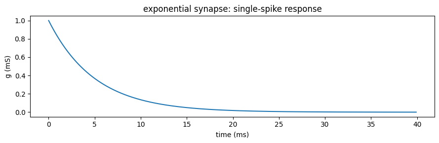
Synapses: temporal filtering of spikes#
A synapse turns a discrete spike train into a continuous signal. The most common is
the exponential synapse: each arriving spike bumps a conductance g that then
decays.
That g ← g + 1 increment is identity-agnostic — it does not matter which
presynaptic neuron fired — and that single fact is what makes the AlignPost
reduction in the next chapter exact. Keep it in mind.
syn = brainpy.state.Expon(1, tau=5. * u.ms,
                          g_initializer=braintools.init.Constant(0. * u.mS))
brainstate.nn.init_all_states(syn)

def syn_step(t):
    with brainstate.environ.context(t=t):
        # a single spike at t = 0, nothing afterwards
        spike = u.math.where(t == 0. * u.ms, 1.0 * u.mS, 0.0 * u.mS)
        return syn(spike)

with brainstate.environ.context(dt=0.1 * u.ms):
    times = u.math.arange(0. * u.ms, 40. * u.ms, brainstate.environ.get_dt())
    g = brainstate.transform.for_loop(syn_step, times)

plt.figure(figsize=(9, 3))
plt.plot(times.to_decimal(u.ms), g.to_decimal(u.mS).squeeze())
plt.xlabel('time (ms)'); plt.ylabel('g (mS)'); plt.title('exponential synapse: single-spike response')
plt.tight_layout(); plt.show()
The family extends well beyond the single exponential — DualExpon and Alpha
add a rise time; AMPA, GABAa, and BioNMDA model receptor kinetics, some
of them nonlinear in the conductance. That linear-vs-nonlinear distinction decides
which projection alignment applies, the central question of the next chapter. (Note
the names: it is GABAa and BioNMDA, not GABA/NMDA.)
Outputs: from conductance to current#
A synapse produces a conductance; an output converts it into the current the postsynaptic neuron actually feels. The choice encodes the biophysics:
CUBA (current-based): \(I = g\). Simple, fast, voltage-independent.
COBA (conductance-based): \(I = g\,(E - V)\), with a reversal potential
E. Self-limiting and biologically realistic — excitatory withE = 0 mV, inhibitory withE = -80 mV.MgBlock (NMDA): COBA plus a voltage-dependent magnesium block.
You do not wire an output by hand — it is one of the four components a projection assembles, which is precisely where we go next.
cuba = brainpy.state.CUBA()
exc = brainpy.state.COBA(E=0. * u.mV)
inh = brainpy.state.COBA(E=-80. * u.mV)
print(cuba, exc, inh)
CUBA(
  scale=Unit("V")
) COBA(
  E=Quantity(0., "mV")
) COBA(
  E=Quantity(-80., "mV")
)
Recap#
Neurons and synapses share one
Dynamicscontract: declare state → allocate →update()→ expose outputs.A neuron integrates current and emits spikes via
get_spike(); synaptic input accumulates additively into its drive.A synapse filters spikes into a conductance; the exponential synapse’s
g ← g + 1increment is identity-agnostic.An output (CUBA / COBA / MgBlock) turns conductance into current.
These four pieces — communication, synapse, output, postsynaptic population — are exactly what a projection composes.
See also#
AlignPre / AlignPost — the keystone — the keystone: how projections wire these pieces across populations, memory-efficiently and exactly.
The state paradigm — the state and
transformmachinery used above.Physical units — the units every parameter carries.
API Reference — the full catalog of neuron, synapse, and output models.