InvSquareGrad

InvSquareGrad#

class braintools.surrogate.InvSquareGrad(alpha=100.0)#

Judge spiking state with the inverse-square surrogate gradient function.

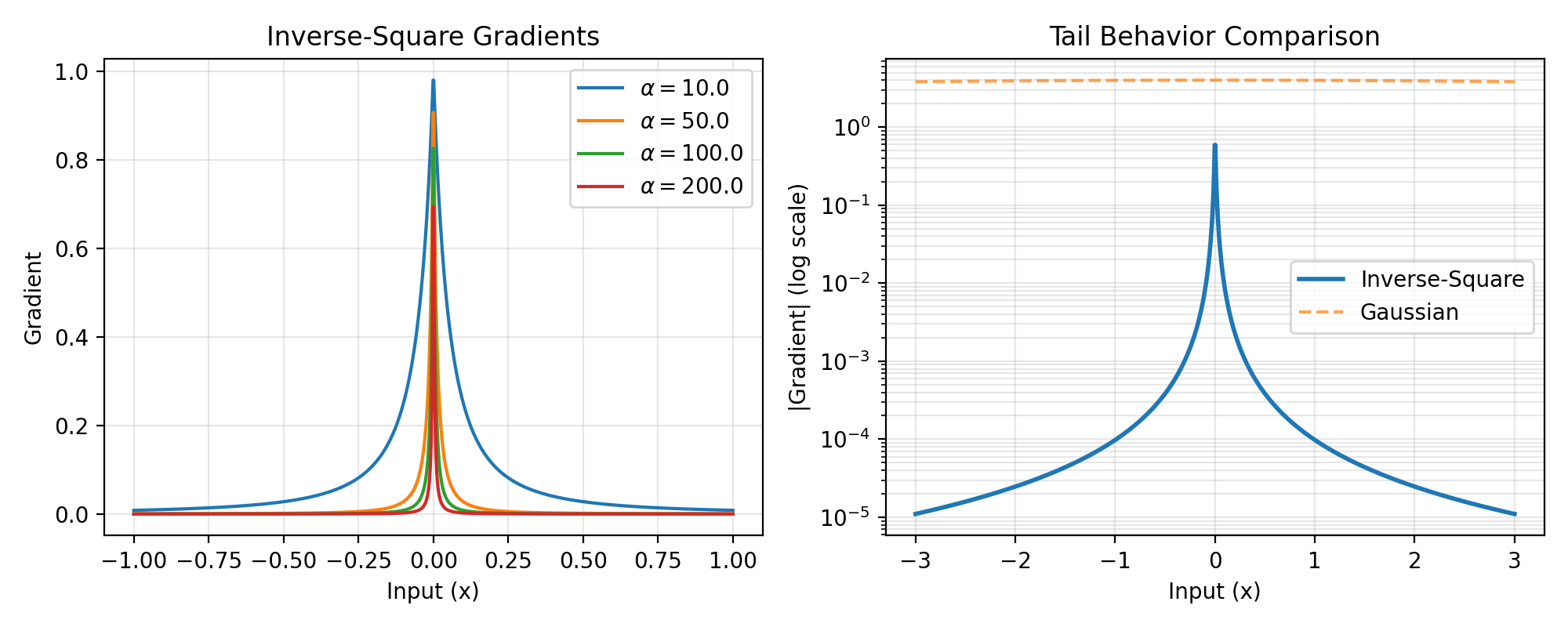
The inverse-square gradient surrogate provides a smooth approximation with a Lorentzian-like profile. It has heavier tails than Gaussian gradients, allowing for gradient flow even far from the threshold, while maintaining a sharp peak at the origin.

The forward function:

\[\begin{split}g(x) = \begin{cases} 1, & x \geq 0 \\ 0, & x < 0 \\ \end{cases}\end{split}\]

Backward gradient:

\[g'(x) = \frac{1}{(\alpha \cdot |x| + 1)^2}\]

This creates a gradient with:

Peak value of 1 at x=0
Power-law decay proportional to 1/x² for large |x|
Width controlled by 1/α

>>> import jax
>>> import jax.numpy as jnp
>>> import brainstate
>>> import braintools.surrogate as surrogate
>>> import matplotlib.pyplot as plt
>>>
>>> xs = jnp.linspace(-1, 1, 1000)
>>> fig, (ax1, ax2) = plt.subplots(1, 2, figsize=(10, 4))
>>>
>>> # Plot gradients for different alpha values
>>> for alpha in [10., 50., 100., 200.]:
>>>     isg_fn = surrogate.InvSquareGrad(alpha=alpha)
>>>     grads = jax.vmap(jax.grad(isg_fn))(xs)
>>>     ax1.plot(xs, grads, label=rf'$\alpha={alpha}$')
>>>
>>> ax1.set_xlabel('Input (x)')
>>> ax1.set_ylabel('Gradient')
>>> ax1.set_title('Inverse-Square Gradients')
>>> ax1.legend()
>>> ax1.grid(True, alpha=0.3)
>>>
>>> # Compare with other surrogate gradients on log scale
>>> xs_wide = jnp.linspace(-3, 3, 1000)
>>> isg_fn = surrogate.InvSquareGrad(alpha=100.)
>>> grads_inv = jax.vmap(jax.grad(isg_fn))(xs_wide)
>>>
>>> # Compare with Gaussian
>>> gg_fn = surrogate.GaussianGrad(sigma=0.1, alpha=1.0)
>>> grads_gauss = jax.vmap(jax.grad(gg_fn))(xs_wide)
>>>
>>> ax2.semilogy(xs_wide, jnp.abs(grads_inv), label='Inverse-Square', linewidth=2)
>>> ax2.semilogy(xs_wide, jnp.abs(grads_gauss), '--', label='Gaussian', alpha=0.7)
>>>
>>> ax2.set_xlabel('Input (x)')
>>> ax2.set_ylabel('|Gradient| (log scale)')
>>> ax2.set_title('Tail Behavior Comparison')
>>> ax2.legend()
>>> ax2.grid(True, alpha=0.3, which="both")
>>> plt.tight_layout()
>>> plt.show()

(Source code, png, hires.png, pdf)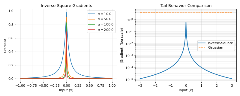

../../_images/braintools-surrogate-InvSquareGrad-1.png

Parameters:

alpha (float, optional) –

Parameter to control gradient sharpness. Default is 100.0.

Larger α creates sharper, more localized gradients
Smaller α creates wider, more distributed gradients
Effective width ≈ 2/α

Examples

>>> import jax
>>> import braintools.surrogate as surrogate
>>>
>>> # Create inverse-square gradient surrogate
>>> isg_fn = surrogate.InvSquareGrad(alpha=100.0)
>>>
>>> # Apply to input
>>> x = jax.numpy.array([-0.1, 0., 0.1])
>>> spikes = isg_fn(x)
>>> print(spikes)
[0. 1. 1.]
>>>
>>> # Compute gradients
>>> grad_fn = jax.grad(lambda x: isg_fn(x).sum())
>>> grads = grad_fn(x)
>>> print(f"Gradients: {grads}")
>>> # Shows heavy-tailed behavior

InvSquareGrad

Contents

InvSquareGrad#