
Ordinary Differential Equation (ODE) Integration Tutorial#
This tutorial demonstrates how to use the ordinary differential equation (ODE) integrators in BrainTools. We’ll cover:
Basic integrators: Euler, RK2, RK3, RK4
Advanced integrators: Embedded methods with error estimation
Specialized methods: Exponential Euler, Strong Stability Preserving
Performance comparison and accuracy analysis
Practical neuroscience examples
All integrators in BrainTools operate on JAX PyTrees and use the global time step from brainstate.environ.
Setup and Imports#
import brainstate
import brainunit as u
import jax
import jax.numpy as jnp
import matplotlib.pyplot as plt
import numpy as np

import braintools

# Set up plotting style
plt.style.use('seaborn-v0_8')
plt.rcParams['figure.figsize'] = (12, 8)
plt.rcParams['font.size'] = 12

# Enable JAX's float64 for better precision in this tutorial
jax.config.update("jax_enable_x64", True)
1. Basic ODE Integrators#
Let’s start with a simple example: the exponential decay equation.
The analytical solution is \(y(t) = y_0 e^{-\lambda t}\).
# Define the ODE
def exponential_decay(y, t, lam=1.0):
    """dy/dt = -lambda * y"""
    return -lam * y


# Analytical solution
def analytical_solution(t, y0=1.0, lam=1.0):
    return y0 * jnp.exp(-lam * t)


# Integration parameters
y0 = 1.0
t_final = 3.0
dt = 0.1
lam = 1.0

# Time array
t_array = jnp.arange(0, t_final + dt, dt)
n_steps = len(t_array) - 1

print(f"Integration from t=0 to t={t_final} with dt={dt}")
print(f"Number of steps: {n_steps}")
Integration from t=0 to t=3.0 with dt=0.1
Number of steps: 30
Euler Method#
The simplest first-order method: \(y_{n+1} = y_n + \Delta t \cdot f(y_n, t_n)\)
# Integrate using Euler method
def integrate_ode(integrator_func, f, y0, t_array, *args):
    """Generic ODE integration function"""
    dt = t_array[1] - t_array[0]
    y = y0

    def step_run(y0, t):
        y1 = integrator_func(f, y0, t, *args)
        return y1, y1

    with brainstate.environ.context(dt=dt):
        y, y_values = brainstate.transform.scan(step_run, y, t_array)
    return jax.block_until_ready(y_values)


# Integrate with Euler method
y_euler = integrate_ode(braintools.quad.ode_euler_step, exponential_decay, y0, t_array, lam)

# Plot results
plt.figure(figsize=(10, 6))
plt.plot(t_array, analytical_solution(t_array, y0, lam), 'k-', linewidth=2, label='Analytical')
plt.plot(t_array, y_euler, 'ro-', markersize=4, label='Euler')
plt.xlabel('Time')
plt.ylabel('y(t)')
plt.title('Exponential Decay: Euler Method')
plt.legend()
plt.grid(True, alpha=0.3)
plt.show()

# Calculate error
analytical = analytical_solution(t_array, y0, lam)
error_euler = jnp.abs(y_euler - analytical)
print(f"Euler method final error: {error_euler[-1]:.6f}")
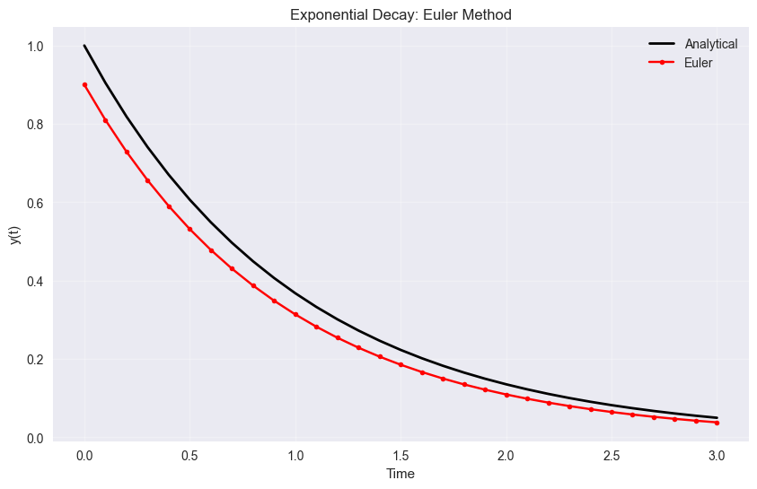
Euler method final error: 0.011635
Runge-Kutta Methods#
Let’s compare different orders of Runge-Kutta methods:
# Integrate with different RK methods
y_rk2 = integrate_ode(braintools.quad.ode_rk2_step, exponential_decay, y0, t_array, lam)
y_rk3 = integrate_ode(braintools.quad.ode_rk3_step, exponential_decay, y0, t_array, lam)
y_rk4 = integrate_ode(braintools.quad.ode_rk4_step, exponential_decay, y0, t_array, lam)

# Plot comparison
plt.figure(figsize=(12, 8))

# Main plot
plt.subplot(2, 1, 1)
plt.plot(t_array, analytical, 'k-', linewidth=3, label='Analytical')
plt.plot(t_array, y_euler, 'ro-', markersize=3, label='Euler (1st order)')
plt.plot(t_array, y_rk2, 'go-', markersize=3, label='RK2 (2nd order)')
plt.plot(t_array, y_rk3, 'bo-', markersize=3, label='RK3 (3rd order)')
plt.plot(t_array, y_rk4, 'mo-', markersize=3, label='RK4 (4th order)')
plt.xlabel('Time')
plt.ylabel('y(t)')
plt.title('Comparison of Runge-Kutta Methods')
plt.legend()
plt.grid(True, alpha=0.3)

# Error plot
plt.subplot(2, 1, 2)
error_rk2 = jnp.abs(y_rk2 - analytical)
error_rk3 = jnp.abs(y_rk3 - analytical)
error_rk4 = jnp.abs(y_rk4 - analytical)

plt.semilogy(t_array, error_euler, 'ro-', markersize=3, label='Euler error')
plt.semilogy(t_array, error_rk2, 'go-', markersize=3, label='RK2 error')
plt.semilogy(t_array, error_rk3, 'bo-', markersize=3, label='RK3 error')
plt.semilogy(t_array, error_rk4, 'mo-', markersize=3, label='RK4 error')
plt.xlabel('Time')
plt.ylabel('Absolute Error (log scale)')
plt.title('Error Comparison')
plt.legend()
plt.grid(True, alpha=0.3)

plt.tight_layout()
plt.show()

# Print final errors
print("Final errors:")
print(f"Euler:  {error_euler[-1]:.2e}")
print(f"RK2:    {error_rk2[-1]:.2e}")
print(f"RK3:    {error_rk3[-1]:.2e}")
print(f"RK4:    {error_rk4[-1]:.2e}")
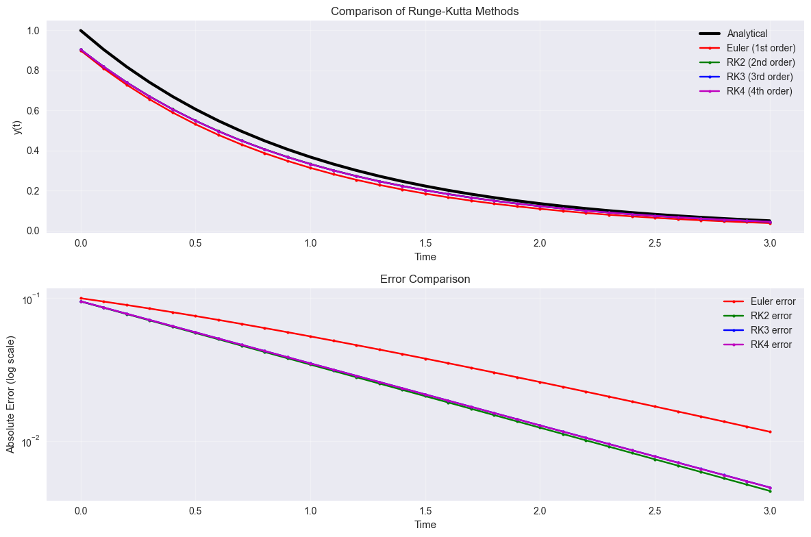
Final errors:
Euler:  1.16e-02
RK2:    4.49e-03
RK3:    4.74e-03
RK4:    4.74e-03
2. Embedded Methods with Error Estimation#
Embedded methods provide automatic error estimation by computing solutions of two different orders. Let’s demonstrate this with the Bogacki-Shampine 2(3) and Dormand-Prince 5(4) methods.
def integrate_ode_with_error(integrator_func, f, y0, t_array, *args):
    """Integration function that returns both solution and error estimates"""
    dt = t_array[1] - t_array[0]
    y = y0

    def step_run(y0, t):
        y1, err = integrator_func(f, y0, t, *args, return_error=True)
        return y1, (y1, err)

    with brainstate.environ.context(dt=dt):
        y, (y_values, errors) = brainstate.transform.scan(step_run, y, t_array)

    return y_values, jax.block_until_ready(errors)
# Integrate with embedded methods
y_rk23, err_rk23 = integrate_ode_with_error(braintools.quad.ode_rk23_step, exponential_decay, y0, t_array, lam)
y_dopri5, err_dopri5 = integrate_ode_with_error(braintools.quad.ode_dopri5_step, exponential_decay, y0, t_array, lam)

# Plot results with error estimates
plt.figure(figsize=(14, 10))

# Solution comparison
plt.subplot(2, 2, 1)
plt.plot(t_array, analytical, 'k-', linewidth=2, label='Analytical')
plt.plot(t_array, y_rk23, 'ro-', markersize=3, label='RK23')
plt.plot(t_array, y_dopri5, 'bo-', markersize=3, label='DOPRI5')
plt.xlabel('Time')
plt.ylabel('y(t)')
plt.title('Embedded Methods Solutions')
plt.legend()
plt.grid(True, alpha=0.3)

# True errors
plt.subplot(2, 2, 2)
true_err_rk23 = jnp.abs(y_rk23 - analytical)
true_err_dopri5 = jnp.abs(y_dopri5 - analytical)
plt.semilogy(t_array, true_err_rk23, 'ro-', markersize=3, label='RK23 true error')
plt.semilogy(t_array, true_err_dopri5, 'bo-', markersize=3, label='DOPRI5 true error')
plt.xlabel('Time')
plt.ylabel('True Error (log scale)')
plt.title('True Errors')
plt.legend()
plt.grid(True, alpha=0.3)

# Error estimates
plt.subplot(2, 2, 3)
plt.semilogy(t_array, jnp.abs(err_rk23), 'ro-', markersize=3, label='RK23 error estimate')
plt.semilogy(t_array, jnp.abs(err_dopri5), 'bo-', markersize=3, label='DOPRI5 error estimate')
plt.xlabel('Time')
plt.ylabel('Error Estimate (log scale)')
plt.title('Built-in Error Estimates')
plt.legend()
plt.grid(True, alpha=0.3)

# Error estimate quality
plt.subplot(2, 2, 4)
ratio_rk23 = true_err_rk23[1:] / jnp.abs(err_rk23[1:])  # Skip first point (zero error)
ratio_dopri5 = true_err_dopri5[1:] / jnp.abs(err_dopri5[1:])
plt.plot(t_array[1:], ratio_rk23, 'ro-', markersize=3, label='RK23 ratio')
plt.plot(t_array[1:], ratio_dopri5, 'bo-', markersize=3, label='DOPRI5 ratio')
plt.axhline(y=1, color='k', linestyle='--', alpha=0.5, label='Perfect estimate')
plt.xlabel('Time')
plt.ylabel('True Error / Error Estimate')
plt.title('Error Estimate Quality')
plt.legend()
plt.grid(True, alpha=0.3)

plt.tight_layout()
plt.show()

print("\nError estimate quality (closer to 1 is better):")
print(f"RK23 mean ratio: {jnp.mean(ratio_rk23):.2f} ± {jnp.std(ratio_rk23):.2f}")
print(f"DOPRI5 mean ratio: {jnp.mean(ratio_dopri5):.2f} ± {jnp.std(ratio_dopri5):.2f}")
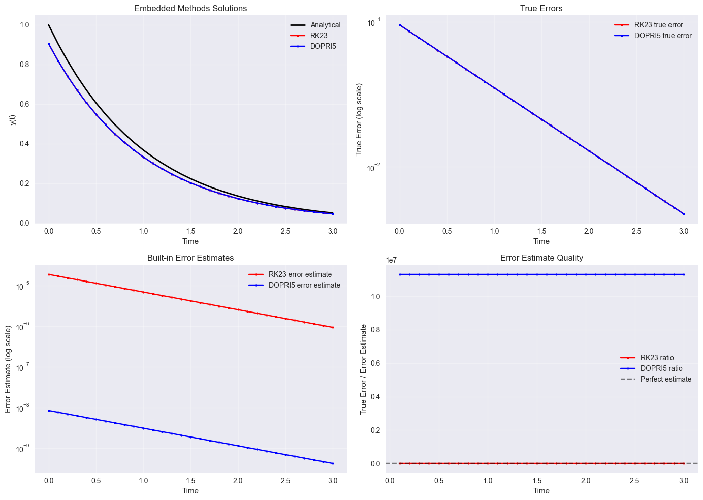
Error estimate quality (closer to 1 is better):
RK23 mean ratio: 5079.29 ± 2.08
DOPRI5 mean ratio: 11312044.76 ± 0.32
# Integrate with embedded methods
y_rk23, err_rk23 = integrate_ode_with_error(braintools.quad.ode_rk23_step, exponential_decay, y0, t_array, lam)
y_dopri5, err_dopri5 = integrate_ode_with_error(braintools.quad.ode_dopri5_step, exponential_decay, y0, t_array, lam)

# Plot results with error estimates
plt.figure(figsize=(14, 10))

# Solution comparison
plt.subplot(2, 2, 1)
plt.plot(t_array, analytical, 'k-', linewidth=2, label='Analytical')
plt.plot(t_array, y_rk23, 'ro-', markersize=3, label='RK23')
plt.plot(t_array, y_dopri5, 'bo-', markersize=3, label='DOPRI5')
plt.xlabel('Time')
plt.ylabel('y(t)')
plt.title('Embedded Methods Solutions')
plt.legend()
plt.grid(True, alpha=0.3)

# True errors
plt.subplot(2, 2, 2)
true_err_rk23 = jnp.abs(y_rk23 - analytical)
true_err_dopri5 = jnp.abs(y_dopri5 - analytical)
plt.semilogy(t_array, true_err_rk23, 'ro-', markersize=3, label='RK23 true error')
plt.semilogy(t_array, true_err_dopri5, 'bo-', markersize=3, label='DOPRI5 true error')
plt.xlabel('Time')
plt.ylabel('True Error (log scale)')
plt.title('True Errors')
plt.legend()
plt.grid(True, alpha=0.3)

# Error estimates
plt.subplot(2, 2, 3)
plt.semilogy(t_array, jnp.abs(err_rk23), 'ro-', markersize=3, label='RK23 error estimate')
plt.semilogy(t_array, jnp.abs(err_dopri5), 'bo-', markersize=3, label='DOPRI5 error estimate')
plt.xlabel('Time')
plt.ylabel('Error Estimate (log scale)')
plt.title('Built-in Error Estimates')
plt.legend()
plt.grid(True, alpha=0.3)

# Error estimate quality
plt.subplot(2, 2, 4)
ratio_rk23 = true_err_rk23[1:] / jnp.abs(err_rk23[1:])  # Skip first point (zero error)
ratio_dopri5 = true_err_dopri5[1:] / jnp.abs(err_dopri5[1:])
plt.plot(t_array[1:], ratio_rk23, 'ro-', markersize=3, label='RK23 ratio')
plt.plot(t_array[1:], ratio_dopri5, 'bo-', markersize=3, label='DOPRI5 ratio')
plt.axhline(y=1, color='k', linestyle='--', alpha=0.5, label='Perfect estimate')
plt.xlabel('Time')
plt.ylabel('True Error / Error Estimate')
plt.title('Error Estimate Quality')
plt.legend()
plt.grid(True, alpha=0.3)

plt.tight_layout()
plt.show()

print("\nError estimate quality (closer to 1 is better):")
print(f"RK23 mean ratio: {jnp.mean(ratio_rk23):.2f} ± {jnp.std(ratio_rk23):.2f}")
print(f"DOPRI5 mean ratio: {jnp.mean(ratio_dopri5):.2f} ± {jnp.std(ratio_dopri5):.2f}")
Error estimate quality (closer to 1 is better):
RK23 mean ratio: 5079.29 ± 2.08
DOPRI5 mean ratio: 11312044.76 ± 0.32
# Test exponential Euler on a stiff problem
def stiff_ode(y, t, lam=50.0):
    """A stiff ODE: dy/dt = -lambda * y with large lambda"""
    return -lam * y


# Parameters for stiff problem
lam_stiff = 50.0
dt_stiff = 0.05  # Relatively large step size
t_final_stiff = 0.5
t_array_stiff = jnp.arange(0, t_final_stiff + dt_stiff, dt_stiff)

# Analytical solution
analytical_stiff = analytical_solution(t_array_stiff, y0, lam_stiff)

# Compare regular Euler vs Exponential Euler
y_euler_stiff = integrate_ode(braintools.quad.ode_euler_step, stiff_ode, y0, t_array_stiff, lam_stiff)
y_expeuler_stiff = integrate_ode(braintools.quad.ode_expeuler_step, stiff_ode, y0, t_array_stiff, lam_stiff)

plt.figure(figsize=(12, 6))

plt.subplot(1, 2, 1)
plt.plot(t_array_stiff, analytical_stiff, 'k-', linewidth=2, label='Analytical')
plt.plot(t_array_stiff, y_euler_stiff, 'ro-', markersize=4, label='Regular Euler')
plt.plot(t_array_stiff, y_expeuler_stiff, 'go-', markersize=4, label='Exponential Euler')
plt.xlabel('Time')
plt.ylabel('y(t)')
plt.title(f'Stiff ODE (λ={lam_stiff}, dt={dt_stiff})')
plt.legend()
plt.grid(True, alpha=0.3)

plt.subplot(1, 2, 2)
error_euler_stiff = jnp.abs(y_euler_stiff - analytical_stiff)
error_expeuler_stiff = jnp.abs(y_expeuler_stiff - analytical_stiff)
plt.semilogy(t_array_stiff, error_euler_stiff, 'ro-', markersize=4, label='Regular Euler error')
plt.semilogy(t_array_stiff, error_expeuler_stiff, 'go-', markersize=4, label='Exponential Euler error')
plt.xlabel('Time')
plt.ylabel('Absolute Error (log scale)')
plt.title('Error Comparison for Stiff ODE')
plt.legend()
plt.grid(True, alpha=0.3)

plt.tight_layout()
plt.show()

print(f"Final errors for stiff ODE:")
print(f"Regular Euler:      {error_euler_stiff[-1]:.2e}")
print(f"Exponential Euler:  {error_expeuler_stiff[-1]:.2e}")
print(f"Improvement factor: {error_euler_stiff[-1] / error_expeuler_stiff[-1]:.1f}x")
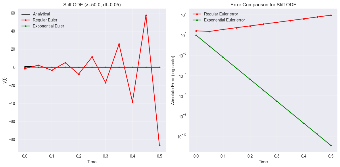
Final errors for stiff ODE:
Regular Euler:      8.65e+01
Exponential Euler:  1.27e-11
Improvement factor: 6785212127633.2x
Strong Stability Preserving RK (SSPRK)#
SSPRK methods are designed to preserve certain stability properties, particularly useful for hyperbolic PDEs and conservation laws.
# Test SSPRK33 method
y_ssprk33 = integrate_ode(braintools.quad.ode_ssprk33_step, exponential_decay, y0, t_array, lam)

plt.figure(figsize=(10, 6))
plt.plot(t_array, analytical, 'k-', linewidth=2, label='Analytical')
plt.plot(t_array, y_rk3, 'bo-', markersize=3, label='Standard RK3')
plt.plot(t_array, y_ssprk33, 'ro-', markersize=3, label='SSPRK(3,3)')
plt.xlabel('Time')
plt.ylabel('y(t)')
plt.title('Strong Stability Preserving RK3')
plt.legend()
plt.grid(True, alpha=0.3)
plt.show()

error_ssprk33 = jnp.abs(y_ssprk33 - analytical)
print(f"SSPRK(3,3) final error: {error_ssprk33[-1]:.2e}")
print(f"Standard RK3 final error: {error_rk3[-1]:.2e}")
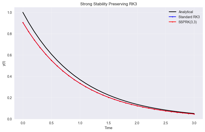
SSPRK(3,3) final error: 4.74e-03
Standard RK3 final error: 4.74e-03
4. Step Size Analysis#
Let’s analyze how the error scales with step size for different methods to verify their theoretical order of accuracy.
# Step size convergence study
dt_values = jnp.array([0.2, 0.1, 0.05, 0.025, 0.0125])
t_final_conv = 1.0

methods = {
    'Euler': braintools.quad.ode_euler_step,
    'RK2': braintools.quad.ode_rk2_step,
    'RK3': braintools.quad.ode_rk3_step,
    'RK4': braintools.quad.ode_rk4_step
}

errors = {name: [] for name in methods.keys()}

for dt in dt_values:
    t_array_conv = jnp.arange(0, t_final_conv + dt, dt)
    analytical_conv = analytical_solution(t_array_conv, y0, lam)

    for name, method in methods.items():
        y_numerical = integrate_ode(method, exponential_decay, y0, t_array_conv, lam)
        error = jnp.abs(y_numerical[-1] - analytical_conv[-1])
        errors[name].append(error)

# Convert to arrays
for name in errors.keys():
    errors[name] = jnp.array(errors[name])

# Plot convergence
plt.figure(figsize=(12, 8))

plt.subplot(1, 2, 1)
for name in methods.keys():
    plt.loglog(dt_values, errors[name], 'o-', markersize=6, label=name)

# Add theoretical slopes
dt_ref = dt_values[2]
error_ref = errors['Euler'][2]
plt.loglog(dt_values, error_ref * (dt_values / dt_ref) ** 1, 'k--', alpha=0.5, label='Order 1')
plt.loglog(dt_values, error_ref * (dt_values / dt_ref) ** 2, 'k:', alpha=0.5, label='Order 2')
plt.loglog(dt_values, error_ref * (dt_values / dt_ref) ** 4, 'k-.', alpha=0.5, label='Order 4')

plt.xlabel('Step Size (dt)')
plt.ylabel('Error at t=1')
plt.title('Convergence Analysis')
plt.legend()
plt.grid(True, alpha=0.3)

# Calculate empirical order of accuracy
plt.subplot(1, 2, 2)
orders = {}
for name in methods.keys():
    order_estimates = []
    for i in range(len(dt_values) - 1):
        order = jnp.log(errors[name][i] / errors[name][i + 1]) / jnp.log(dt_values[i] / dt_values[i + 1])
        order_estimates.append(order)
    orders[name] = jnp.array(order_estimates)
    plt.plot(
        dt_values[:-1],
        order_estimates,
        'o-',
        markersize=6,
        label=f'{name} (avg: {np.mean(order_estimates):.2f})'
    )

plt.axhline(y=1, color='k', linestyle='--', alpha=0.5, label='Order 1')
plt.axhline(y=2, color='k', linestyle=':', alpha=0.5, label='Order 2')
plt.axhline(y=4, color='k', linestyle='-.', alpha=0.5, label='Order 4')
plt.xlabel('Step Size (dt)')
plt.ylabel('Empirical Order of Accuracy')
plt.title('Measured Order of Accuracy')
plt.legend()
plt.grid(True, alpha=0.3)

plt.tight_layout()
plt.show()

print("Average empirical orders of accuracy:")
for name in methods.keys():
    print(f"{name}: {jnp.mean(orders[name]):.2f}")
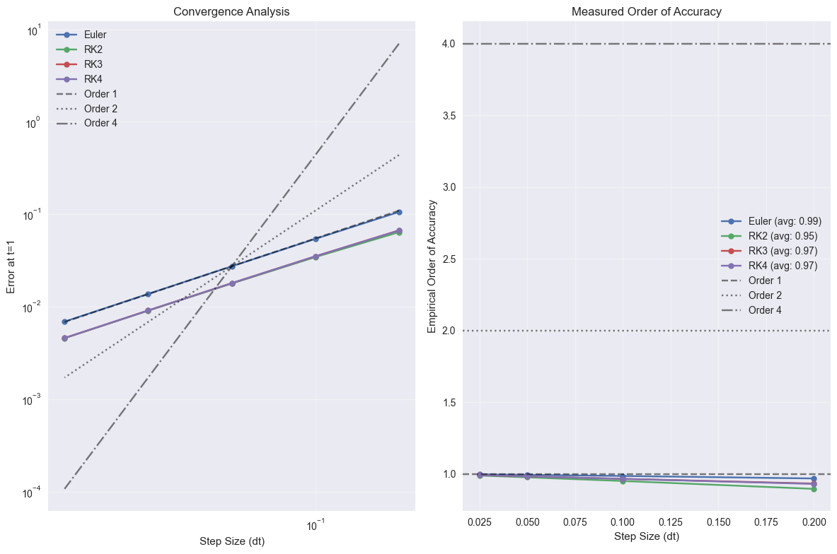
Average empirical orders of accuracy:
Euler: 0.99
RK2: 0.95
RK3: 0.97
RK4: 0.97
5. Practical Neuroscience Example: Hodgkin-Huxley Neuron#
Let’s solve a simplified version of the Hodgkin-Huxley equations for a single neuron compartment.
class HH(brainstate.nn.Dynamics):
    def __init__(
        self,
        in_size,
        ENa=50. * u.mV,
        gNa=120. * u.mS / u.cm ** 2,
        EK=-77. * u.mV,
        gK=36. * u.mS / u.cm ** 2,
        EL=-54.387 * u.mV,
        gL=0.03 * u.mS / u.cm ** 2,
        V_th=20. * u.mV,
        C=1.0 * u.uF / u.cm ** 2,
        method=braintools.quad.ode_rk87_dopri_step,
    ):
        # initialization
        super().__init__(in_size)

        # parameters
        self.ENa = ENa
        self.EK = EK
        self.EL = EL
        self.gNa = gNa
        self.gK = gK
        self.gL = gL
        self.C = C
        self.V_th = V_th
        self.method = method

    # m channel
    m_alpha = lambda self, V: 1. / u.math.exprel(-(V / u.mV + 40) / 10)
    m_beta = lambda self, V: 4.0 * jnp.exp(-(V / u.mV + 65) / 18)
    m_inf = lambda self, V: self.m_alpha(V) / (self.m_alpha(V) + self.m_beta(V))
    dm = lambda self, m, t, V: (self.m_alpha(V) * (1 - m) - self.m_beta(V) * m) / u.ms

    # h channel
    h_alpha = lambda self, V: 0.07 * jnp.exp(-(V / u.mV + 65) / 20.)
    h_beta = lambda self, V: 1 / (1 + jnp.exp(-(V / u.mV + 35) / 10))
    h_inf = lambda self, V: self.h_alpha(V) / (self.h_alpha(V) + self.h_beta(V))
    dh = lambda self, h, t, V: (self.h_alpha(V) * (1 - h) - self.h_beta(V) * h) / u.ms

    # n channel
    n_alpha = lambda self, V: 0.1 / u.math.exprel(-(V / u.mV + 55) / 10)
    n_beta = lambda self, V: 0.125 * jnp.exp(-(V / u.mV + 65) / 80)
    n_inf = lambda self, V: self.n_alpha(V) / (self.n_alpha(V) + self.n_beta(V))
    dn = lambda self, n, t, V: (self.n_alpha(V) * (1 - n) - self.n_beta(V) * n) / u.ms

    def init_state(self, batch_size=None):
        self.V = brainstate.HiddenState(jnp.ones(self.varshape) * -65. * u.mV)
        self.m = brainstate.HiddenState(self.m_inf(self.V.value))
        self.h = brainstate.HiddenState(self.h_inf(self.V.value))
        self.n = brainstate.HiddenState(self.n_inf(self.V.value))

    def dV(self, V, t, m, h, n, I):
        I = self.sum_current_inputs(I, V)
        I_Na = (self.gNa * m * m * m * h) * (V - self.ENa)
        n2 = n * n
        I_K = (self.gK * n2 * n2) * (V - self.EK)
        I_leak = self.gL * (V - self.EL)
        dVdt = (- I_Na - I_K - I_leak + I) / self.C
        return dVdt

    def derivative(self, state, t, inp):
        V, m, h, n = state
        dV = self.dV(V, t, m, h, n, inp)
        dm = self.dm(m, t, V)
        dh = self.dh(h, t, V)
        dn = self.dn(n, t, V)
        return dV, dm, dh, dn

    def update(self, x=0. * u.mA / u.cm ** 2):
        t = brainstate.environ.get('t')
        V, m, h, n = self.method(
            self.derivative,
            (self.V.value, self.m.value, self.h.value, self.n.value),
            0. * u.ms,
            x
        )

        V = self.sum_delta_inputs(init=V)
        spike = jnp.logical_and(self.V.value < self.V_th, V >= self.V_th)
        self.V.value = V
        self.m.value = m
        self.h.value = h
        self.n.value = n
        return spike

    def step_run(self, i, inp):
        with brainstate.environ.context(t=i * brainstate.environ.get_dt(), i=i):
            spike = self.update(inp)
            return self.V.value, self.m.value, self.h.value, self.n.value
brainstate.environ.set(dt=0.01 * u.ms)
indices = np.arange(10000)
t_array_hh = indices * brainstate.environ.get_dt()

hh = HH(in_size=1, method=braintools.quad.ode_rk4_step)
hh.init_state()
I_ext_array = brainstate.random.uniform(1., 10., indices.shape) * u.uA / u.cm ** 2
V_hh, m_hh, h_hh, n_hh = brainstate.transform.for_loop(hh.step_run, indices, I_ext_array)
V_hh = jax.block_until_ready(V_hh)

# Plot results
plt.figure(figsize=(14, 10))

plt.subplot(3, 1, 1)
plt.plot(t_array_hh, V_hh, 'b-', linewidth=2)
plt.ylabel('Membrane Potential (mV)')
plt.title('Hodgkin-Huxley Neuron Model')
plt.grid(True, alpha=0.3)

plt.subplot(3, 1, 2)
plt.plot(t_array_hh, m_hh, 'r-', label='m (Na activation)', linewidth=2)
plt.plot(t_array_hh, h_hh, 'g-', label='h (Na inactivation)', linewidth=2)
plt.plot(t_array_hh, n_hh, 'b-', label='n (K activation)', linewidth=2)
plt.ylabel('Gating Variables')
plt.legend()
plt.grid(True, alpha=0.3)

plt.subplot(3, 1, 3)
plt.plot(t_array_hh, I_ext_array, 'k-', linewidth=2)
plt.xlabel('Time (ms)')
plt.ylabel('Injected Current (μA/cm²)')
plt.grid(True, alpha=0.3)

plt.tight_layout()
plt.show()

print(f"Peak membrane potential: {V_hh.max():.1f}")
print(f"Resting potential: {V_hh[0]:.1f}")
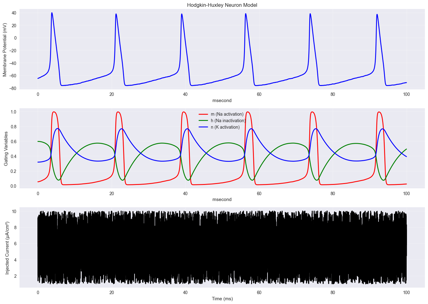
Peak membrane potential: 39.7 * mvolt
Resting potential: ArrayImpl([-64.9]) * mvolt
6. Performance Considerations#
Let’s compare the computational efficiency of different methods.
import time


# Timing test setup
def time_integrator(integrator_func, f, y0, n_steps, dt_val, *args):
    """Time an integrator over n_steps"""
    t_array_timing = jnp.arange(0, n_steps * dt_val, dt_val)

    # Warm-up run (for JAX compilation)
    _ = integrate_ode(integrator_func, f, y0, t_array_timing[:10], *args)

    # Actual timing
    start_time = time.time()
    result = integrate_ode(integrator_func, f, y0, t_array_timing, *args)
    end_time = time.time()

    return end_time - start_time, result[-1]


# Timing parameters
n_steps_timing = 1000
dt_timing = 0.01

timing_methods = {
    'Euler': braintools.quad.ode_euler_step,
    'RK2': braintools.quad.ode_rk2_step,
    'RK4': braintools.quad.ode_rk4_step,
    'DOPRI5': braintools.quad.ode_dopri5_step,
}

times = {}
final_values = {}

print("Timing integrators over {} steps...".format(n_steps_timing))
for name, method in timing_methods.items():
    elapsed, final_val = time_integrator(method, exponential_decay, y0, n_steps_timing, dt_timing, lam)
    times[name] = elapsed
    final_values[name] = final_val
    print(f"{name:8s}: {elapsed:.4f} seconds, final value: {final_val:.6f}")

# Efficiency analysis
euler_time = times['Euler']
print("\nRelative timing (vs Euler):")
for name, time_val in times.items():
    print(f"{name:8s}: {time_val / euler_time:.2f}x")

# Accuracy per computational cost
analytical_final = analytical_solution(n_steps_timing * dt_timing, y0, lam)
print("\nAccuracy per computational cost:")
for name in timing_methods.keys():
    error = jnp.abs(final_values[name] - analytical_final)
    efficiency = 1.0 / (error * times[name])  # Higher is better
    print(f"{name:8s}: error={error:.2e}, efficiency={efficiency:.2e}")
Timing integrators over 1000 steps...
Euler   : 0.0450 seconds, final value: 0.000043
RK2     : 0.0341 seconds, final value: 0.000045
RK4     : 0.0388 seconds, final value: 0.000045
DOPRI5  : 0.0473 seconds, final value: 0.000045

Relative timing (vs Euler):
Euler   : 1.00x
RK2     : 0.76x
RK4     : 0.86x
DOPRI5  : 1.05x

Accuracy per computational cost:
Euler   : error=2.23e-06, efficiency=9.97e+06
RK2     : error=7.62e-09, efficiency=3.85e+09
RK4     : error=3.81e-14, efficiency=6.76e+14
DOPRI5  : error=1.27e-17, efficiency=1.66e+18
Summary#
This tutorial covered the key ODE integrators available in BrainTools:
Basic Methods:
Euler: First-order, simple but less accurate
RK2/RK3/RK4: Higher-order methods with better accuracy
Advanced Methods:
Embedded methods (RK23, DOPRI5): Automatic error estimation
Exponential Euler: Better stability for stiff problems
SSPRK: Strong stability preserving properties
Key Guidelines:
For most problems: Use RK4 or DOPRI5
For stiff problems: Try exponential Euler
For adaptive stepping: Use embedded methods with error estimates
For efficiency: Start with RK2 or RK4 depending on accuracy needs
BrainTools Features:
All methods work with JAX PyTrees
Global time step management via
brainstate.environAutomatic differentiation compatible
Unit-aware computations with
brainunit
Choose your integrator based on the trade-off between accuracy, stability, and computational cost for your specific problem.