Tutorial 2: ScipyOptimizer Tutorial

This tutorial demonstrates how to use the ScipyOptimizer from BrainTools for gradient-based optimization. The ScipyOptimizer provides a convenient wrapper around SciPy’s optimization methods with automatic differentiation via JAX, support for complex parameter structures, and seamless integration with BrainUnit quantities.

Introduction and Setup

The ScipyOptimizer is designed for gradient-based optimization where derivatives can be computed automatically via JAX. It’s particularly useful for:

• Smooth, differentiable objective functions

• Neural network parameter optimization

• Physics-based models with analytical gradients

• Problems where gradient information is reliable

Key advantages over derivative-free methods:

• Faster convergence for smooth problems

• Higher precision solutions

• Automatic gradients via JAX

• Mature algorithms from SciPy

Let’s start by importing the necessary libraries:

# Core imports
import jax
import jax.numpy as jnp
import numpy as np
import matplotlib.pyplot as plt
from scipy.optimize import OptimizeResult

# BrainTools imports
import braintools as bts
import brainunit as u
import brainstate as bst

# Set up plotting
plt.style.use('default')
plt.rcParams['figure.figsize'] = (10, 6)

print("BrainTools version:", bts.__version__)
print("JAX version:", jax.__version__)

BrainTools version: 0.0.12
JAX version: 0.7.1

First, let’s check if SciPy is installed (it’s required for the optimizer to work):

try:
    import scipy
    from scipy.optimize import minimize
    print(f"SciPy version: {scipy.__version__}")
    print("✓ SciPy is available")
except ImportError:
    print("❌ SciPy is not installed. Please install it with:")
    print("   pip install scipy")
    raise

SciPy version: 1.14.1
✓ SciPy is available

Basic Usage: Scalar Parameters

Let’s start with a simple example: optimizing a quadratic function with two scalar parameters.

# Define a simple quadratic loss function
def quadratic_loss(x, y):
    """
    Simple quadratic function with known minimum at (2, -1).
    
    Args:
        x, y: Scalar parameters
        
    Returns:
        Scalar loss value
    """
    return (x - 2.0)**2 + (y + 1.0)**2

# Define bounds for each parameter: (min, max)
bounds = [
    (-5.0, 5.0),  # bounds for x
    (-3.0, 3.0),  # bounds for y
]

# Create the optimizer
optimizer = bts.optim.ScipyOptimizer(
    loss_fun=quadratic_loss,
    bounds=bounds,
    method='L-BFGS-B'  # Limited-memory BFGS with bounds
)

print("Optimizer created successfully!")
print(f"Method: {optimizer.method}")
print(f"Bounds structure: {type(bounds).__name__}")

Optimizer created successfully!
Method: L-BFGS-B
Bounds structure: list

# Run the optimization
result = optimizer.minimize(n_iter=3)  # Try 3 random starting points

print(f"\nOptimization completed!")
print(f"Success: {result.success}")
print(f"Message: {result.message}")
print(f"Optimal parameters: x={result.x[0]:.6f}, y={result.x[1]:.6f}")
print(f"True optimum: x=2.0, y=-1.0")
print(f"Final loss: {result.fun:.10f}")
print(f"Function evaluations: {result.nfev}")
print(f"Gradient evaluations: {result.njev}")

Optimization completed!
Success: True
Message: CONVERGENCE: NORM_OF_PROJECTED_GRADIENT_<=_PGTOL
Optimal parameters: x=2.000000, y=-1.000000
True optimum: x=2.0, y=-1.0
Final loss: 0.0000000000
Function evaluations: 4
Gradient evaluations: 4

# Visualize the optimization landscape and result
fig, (ax1, ax2) = plt.subplots(1, 2, figsize=(14, 5))

# Plot the function landscape
x_range = np.linspace(-5, 5, 100)
y_range = np.linspace(-3, 3, 100)
X, Y = np.meshgrid(x_range, y_range)
Z = (X - 2.0)**2 + (Y + 1.0)**2

contour = ax1.contourf(X, Y, Z, levels=30, cmap='viridis', alpha=0.7)
ax1.contour(X, Y, Z, levels=20, colors='black', alpha=0.3, linewidths=0.5)
plt.colorbar(contour, ax=ax1)

# Mark the true optimum and found optimum
ax1.plot(2.0, -1.0, 'r*', markersize=15, label='True optimum')
ax1.plot(result.x[0], result.x[1], 'bo', markersize=10, label='Found optimum')

ax1.set_xlabel('x')
ax1.set_ylabel('y')
ax1.set_title('Quadratic Function Landscape')
ax1.legend()
ax1.grid(True, alpha=0.3)

# Show convergence (we don't have iteration history, so show final result)
ax2.bar(['Final Loss'], [result.fun], color='blue', alpha=0.7)
ax2.set_ylabel('Loss Value')
ax2.set_title('Optimization Result')
ax2.set_yscale('log')
ax2.grid(True, alpha=0.3)

plt.tight_layout()
plt.show()

print(f"Distance from true optimum: {np.sqrt((result.x[0] - 2.0)**2 + (result.x[1] + 1.0)**2):.2e}")

C:\Users\adadu\AppData\Local\Temp\ipykernel_59268\1560779676.py:28: UserWarning: Data has no positive values, and therefore cannot be log-scaled.
  ax2.set_yscale('log')

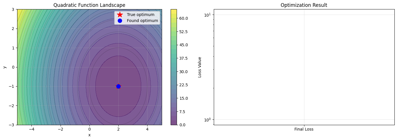
Distance from true optimum: 0.00e+00

Multi-dimensional Array Parameters

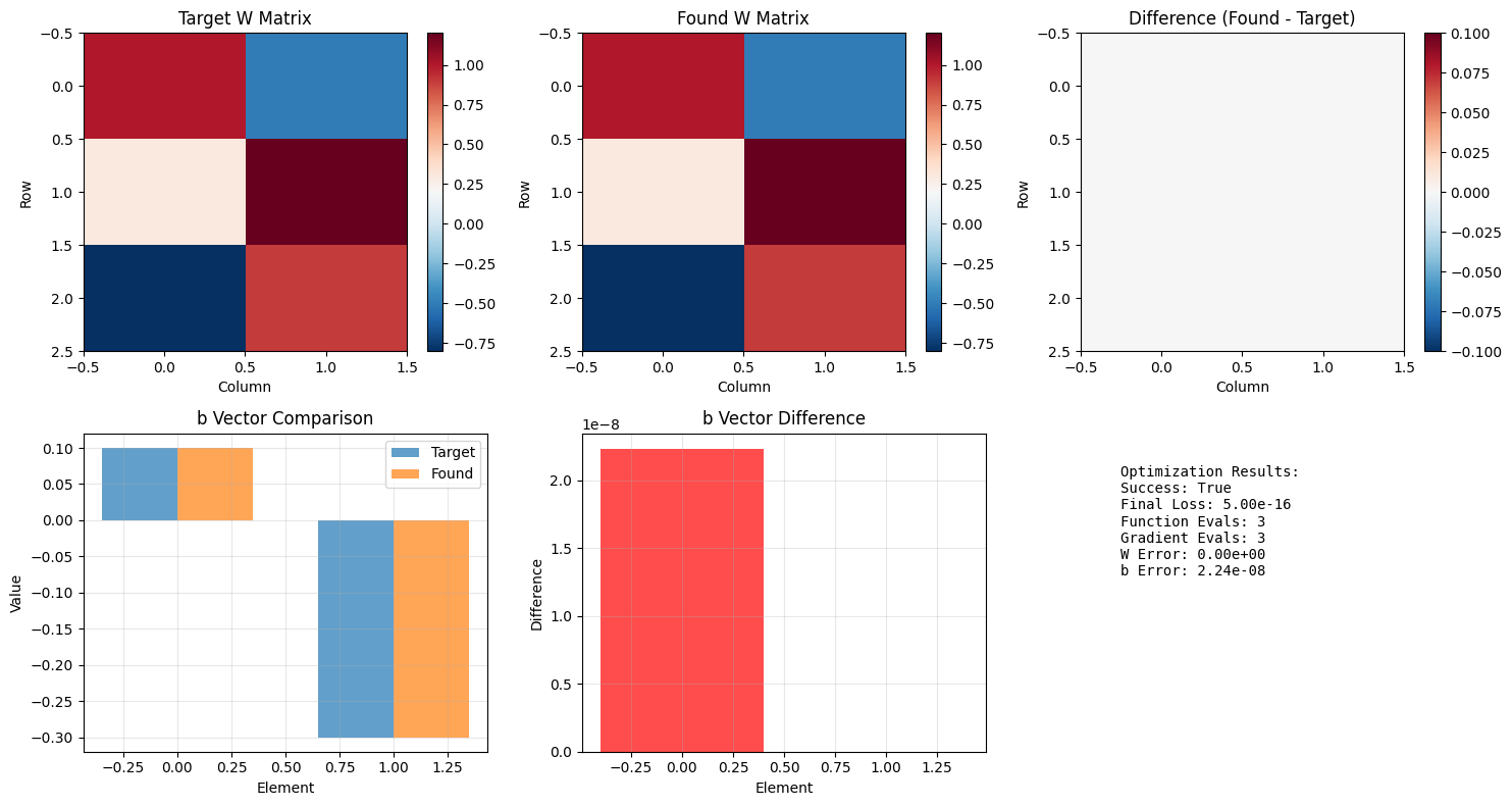
The ScipyOptimizer can handle multi-dimensional arrays as parameters. Let’s optimize a function that takes matrix parameters.

# Define a loss function with matrix parameters
def matrix_frobenius_loss(W, b):
    """
    Find matrix W and vector b that minimize Frobenius norm from targets.
    
    Args:
        W: Matrix parameter of shape (3, 2)
        b: Vector parameter of shape (2,)
        
    Returns:
        Scalar loss (Frobenius norm squared)
    """
    W_target = jnp.array([[1.0, -0.5], [0.3, 1.2], [-0.8, 0.9]])
    b_target = jnp.array([0.1, -0.3])
    
    W_diff = W - W_target
    b_diff = b - b_target
    
    return jnp.sum(W_diff**2) + jnp.sum(b_diff**2)

# Define bounds for array parameters
bounds = [
    (jnp.full((3, 2), -2.0), jnp.full((3, 2), 2.0)),  # bounds for W (3x2 matrix)
    (jnp.full(2, -1.0), jnp.full(2, 1.0)),            # bounds for b (2D vector)
]

# Create optimizer
matrix_optimizer = bts.optim.ScipyOptimizer(
    loss_fun=matrix_frobenius_loss,
    bounds=bounds,
    method='L-BFGS-B'  # Good for smooth, bounded problems
)

print("Multi-dimensional optimizer created!")
print(f"W parameter shape: {bounds[0][0].shape}")
print(f"b parameter shape: {bounds[1][0].shape}")

Multi-dimensional optimizer created!
W parameter shape: (3, 2)
b parameter shape: (2,)

# Run optimization
matrix_result = matrix_optimizer.minimize(n_iter=5)

W_best, b_best = matrix_result.x
print(f"\nOptimization completed!")
print(f"Success: {matrix_result.success}")
print(f"Function evaluations: {matrix_result.nfev}")

print(f"\nOptimal W matrix:")
print(W_best)
print(f"\nOptimal b vector:")
print(b_best)

# Compare with targets
W_target = jnp.array([[1.0, -0.5], [0.3, 1.2], [-0.8, 0.9]])
b_target = jnp.array([0.1, -0.3])
print(f"\nTarget W matrix:")
print(W_target)
print(f"\nTarget b vector:")
print(b_target)

print(f"\nFinal loss: {matrix_result.fun:.10f}")
print(f"W error (Frobenius): {jnp.linalg.norm(W_best - W_target):.2e}")
print(f"b error (L2): {jnp.linalg.norm(b_best - b_target):.2e}")

Optimization completed!
Success: True
Function evaluations: 3

Optimal W matrix:
[[ 1.  -0.5]
 [ 0.3  1.2]
 [-0.8  0.9]]

Optimal b vector:
[ 0.10000002 -0.3       ]

Target W matrix:
[[ 1.  -0.5]
 [ 0.3  1.2]
 [-0.8  0.9]]

Target b vector:
[ 0.1 -0.3]

Final loss: 0.0000000000
W error (Frobenius): 0.00e+00
b error (L2): 2.24e-08

# Visualize the matrix optimization results
fig, axes = plt.subplots(2, 3, figsize=(15, 8))

# Plot W matrix: target, found, and difference
im1 = axes[0, 0].imshow(W_target, cmap='RdBu_r', aspect='auto')
axes[0, 0].set_title('Target W Matrix')
axes[0, 0].set_xlabel('Column')
axes[0, 0].set_ylabel('Row')
plt.colorbar(im1, ax=axes[0, 0])

im2 = axes[0, 1].imshow(W_best, cmap='RdBu_r', aspect='auto')
axes[0, 1].set_title('Found W Matrix')
axes[0, 1].set_xlabel('Column')
axes[0, 1].set_ylabel('Row')
plt.colorbar(im2, ax=axes[0, 1])

W_diff = W_best - W_target
im3 = axes[0, 2].imshow(W_diff, cmap='RdBu_r', aspect='auto')
axes[0, 2].set_title('Difference (Found - Target)')
axes[0, 2].set_xlabel('Column')
axes[0, 2].set_ylabel('Row')
plt.colorbar(im3, ax=axes[0, 2])

# Plot b vector: target, found, and difference
x_pos = np.arange(len(b_target))
width = 0.35

axes[1, 0].bar(x_pos - width/2, b_target, width, label='Target', alpha=0.7)
axes[1, 0].bar(x_pos + width/2, b_best, width, label='Found', alpha=0.7)
axes[1, 0].set_xlabel('Element')
axes[1, 0].set_ylabel('Value')
axes[1, 0].set_title('b Vector Comparison')
axes[1, 0].legend()
axes[1, 0].grid(True, alpha=0.3)

# Plot the difference in b
b_diff = b_best - b_target
axes[1, 1].bar(x_pos, b_diff, alpha=0.7, color='red')
axes[1, 1].set_xlabel('Element')
axes[1, 1].set_ylabel('Difference')
axes[1, 1].set_title('b Vector Difference')
axes[1, 1].grid(True, alpha=0.3)

# Plot optimization info
info_text = f"""Optimization Results:
Success: {matrix_result.success}
Final Loss: {matrix_result.fun:.2e}
Function Evals: {matrix_result.nfev}
Gradient Evals: {matrix_result.njev}
W Error: {jnp.linalg.norm(W_diff):.2e}
b Error: {jnp.linalg.norm(b_diff):.2e}"""

axes[1, 2].text(0.1, 0.9, info_text, transform=axes[1, 2].transAxes, 
                verticalalignment='top', fontsize=10, fontfamily='monospace')
axes[1, 2].set_xlim(0, 1)
axes[1, 2].set_ylim(0, 1)
axes[1, 2].axis('off')

plt.tight_layout()
plt.show()

Named Parameters with Dictionary Bounds

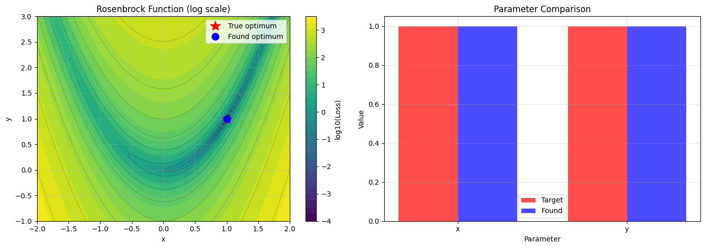
For better organization, especially with many parameters, you can use dictionary bounds to give meaningful names to your parameters.

# Define a loss function that accepts named parameters
def rosenbrock_loss(**params):
    """
    The famous Rosenbrock function with named parameters.
    Global minimum at x=1, y=1 with value 0.
    
    Args:
        **params: Dictionary with keys 'x' and 'y'
        
    Returns:
        Scalar loss value
    """
    x, y = params['x'], params['y']
    a, b = 1.0, 100.0
    return (a - x)**2 + b * (y - x**2)**2

# Define named bounds
named_bounds = {
    'x': (-2.0, 2.0),
    'y': (-1.0, 3.0)
}

# Create optimizer with named parameters
named_optimizer = bts.optim.ScipyOptimizer(
    loss_fun=rosenbrock_loss,
    bounds=named_bounds,
    method='L-BFGS-B'
)

print("Named parameter optimizer created!")
print(f"Parameters: {list(named_bounds.keys())}")

Named parameter optimizer created!
Parameters: ['x', 'y']

# Run optimization
named_result = named_optimizer.minimize(n_iter=5)

print(f"\nOptimization completed!")
print(f"Success: {named_result.success}")
print(f"Function evaluations: {named_result.nfev}")
print(f"Gradient evaluations: {named_result.njev}")

print(f"\nOptimal parameters:")
for param_name, value in named_result.x.items():
    print(f"  {param_name}: {value:.6f}")

print(f"\nTrue optimal values:")
print(f"  x: 1.000000")
print(f"  y: 1.000000")

print(f"\nFinal loss: {named_result.fun:.10f}")
print(f"Distance from optimum: {np.sqrt((named_result.x['x'] - 1.0)**2 + (named_result.x['y'] - 1.0)**2):.2e}")

Optimization completed!
Success: True
Function evaluations: 30
Gradient evaluations: 30

Optimal parameters:
  x: 1.000000
  y: 1.000000

True optimal values:
  x: 1.000000
  y: 1.000000

Final loss: 0.0000000000
Distance from optimum: 2.67e-07

# Visualize the Rosenbrock function and optimization result
fig, (ax1, ax2) = plt.subplots(1, 2, figsize=(14, 5))

# Plot the Rosenbrock function landscape
x_range = np.linspace(-2, 2, 100)
y_range = np.linspace(-1, 3, 100)
X, Y = np.meshgrid(x_range, y_range)
Z = (1 - X)**2 + 100 * (Y - X**2)**2

# Use log scale for better visualization
Z_log = np.log10(Z + 1e-10)
contour = ax1.contourf(X, Y, Z_log, levels=30, cmap='viridis')
ax1.contour(X, Y, Z_log, levels=20, colors='black', alpha=0.3, linewidths=0.5)
plt.colorbar(contour, ax=ax1, label='log10(Loss)')

# Mark the true optimum and found optimum
ax1.plot(1.0, 1.0, 'r*', markersize=15, label='True optimum')
ax1.plot(named_result.x['x'], named_result.x['y'], 'bo', markersize=10, label='Found optimum')

ax1.set_xlabel('x')
ax1.set_ylabel('y')
ax1.set_title('Rosenbrock Function (log scale)')
ax1.legend()
ax1.grid(True, alpha=0.3)

# Plot parameter values
param_names = list(named_result.x.keys())
param_values = [named_result.x[name] for name in param_names]
target_values = [1.0, 1.0]

x_pos = np.arange(len(param_names))
width = 0.35

ax2.bar(x_pos - width/2, target_values, width, label='Target', alpha=0.7, color='red')
ax2.bar(x_pos + width/2, param_values, width, label='Found', alpha=0.7, color='blue')

ax2.set_xlabel('Parameter')
ax2.set_ylabel('Value')
ax2.set_title('Parameter Comparison')
ax2.set_xticks(x_pos)
ax2.set_xticklabels(param_names)
ax2.legend()
ax2.grid(True, alpha=0.3)

plt.tight_layout()
plt.show()

Working with BrainUnit Quantities

The ScipyOptimizer seamlessly integrates with BrainUnit quantities, allowing you to optimize parameters with physical units.

# Define a loss function for neuron model parameters with units
def neuron_model_loss(tau_m, V_th, V_reset, I_ext):
    """
    Loss function for fitting a neuron model to target parameters.
    
    Args:
        tau_m: Membrane time constant (scalar)
        V_th: Threshold voltage (scalar)
        V_reset: Reset voltage (scalar)
        I_ext: External current (scalar)
        
    Returns:
        Scalar loss representing deviation from target behavior
    """
    # Target values (without units - optimizer handles unit conversion)
    tau_target = 20.0    # ms
    V_th_target = -50.0  # mV
    V_reset_target = -70.0  # mV
    I_target = 100.0     # pA
    
    # Compute normalized squared differences
    tau_loss = ((tau_m - tau_target) / 10.0)**2
    V_th_loss = ((V_th - V_th_target) / 10.0)**2
    V_reset_loss = ((V_reset - V_reset_target) / 10.0)**2
    I_loss = ((I_ext - I_target) / 50.0)**2
    
    return tau_loss + V_th_loss + V_reset_loss + I_loss

# Define bounds with units
unit_bounds = {
    'tau_m': (5.0 * u.ms, 50.0 * u.ms),
    'V_th': (-80.0 * u.mV, -30.0 * u.mV),
    'V_reset': (-90.0 * u.mV, -60.0 * u.mV),
    'I_ext': (10.0 * u.pA, 200.0 * u.pA)
}

# Create optimizer
unit_optimizer = bts.optim.ScipyOptimizer(
    loss_fun=neuron_model_loss,
    bounds=unit_bounds,
    method='L-BFGS-B'
)

print("Neuron parameter optimizer with units created!")
for name, (low, high) in unit_bounds.items():
    print(f"  {name}: {low} to {high}")

Neuron parameter optimizer with units created!
  tau_m: 5.0 * msecond to 50.0 * msecond
  V_th: -80.0 * mvolt to -30.0 * mvolt
  V_reset: -90.0 * mvolt to -60.0 * mvolt
  I_ext: 10.0 * pamp to 200.0 * pamp

# Run optimization with units
unit_result = unit_optimizer.minimize(n_iter=3)

print(f"\nOptimization completed!")
print(f"Success: {unit_result.success}")
print(f"Function evaluations: {unit_result.nfev}")

print(f"\nOptimal neuron parameters:")
for param_name, value in unit_result.x.items():
    print(f"  {param_name}: {value:.6f}")

print(f"\nTarget parameters:")
print(f"  tau_m: 20.0")
print(f"  V_th: -50.0")
print(f"  V_reset: -70.0")
print(f"  I_ext: 100.0")

print(f"\nFinal loss: {unit_result.fun:.10f}")

# Note: The optimizer works with dimensionless values internally
# but maintains the parameter structure

Optimization completed!
Success: True
Function evaluations: 9

Optimal neuron parameters:
  I_ext: 100.000000
  V_reset: -70.000000
  V_th: -50.000000
  tau_m: 20.000000

Target parameters:
  tau_m: 20.0
  V_th: -50.0
  V_reset: -70.0
  I_ext: 100.0

Final loss: 0.0000000000

# Visualize neuron parameter optimization results
fig, axes = plt.subplots(2, 2, figsize=(12, 8))
axes = axes.flatten()

# Define target values and units for visualization
targets = {
    'tau_m': (20.0, 'ms'),
    'V_th': (-50.0, 'mV'),
    'V_reset': (-70.0, 'mV'),
    'I_ext': (100.0, 'pA')
}

for i, (param_name, (target_val, unit)) in enumerate(targets.items()):
    found_val = unit_result.x[param_name]
    
    # Plot comparison
    axes[i].bar(['Target', 'Found'], [target_val, found_val], 
               color=['red', 'blue'], alpha=0.7)
    axes[i].set_ylabel(f'{param_name} ({unit})')
    axes[i].set_title(f'{param_name} Optimization')
    axes[i].grid(True, alpha=0.3)
    
    # Add value labels on bars
    axes[i].text(0, target_val, f'{target_val:.1f}', ha='center', va='bottom')
    axes[i].text(1, found_val, f'{found_val:.1f}', ha='center', va='bottom')
    
    # Add error information
    error = abs(found_val - target_val)
    rel_error = error / abs(target_val) * 100
    axes[i].text(0.5, max(target_val, found_val) * 1.1, 
                f'Error: {error:.2f} ({rel_error:.2f}%)', 
                ha='center', va='bottom', fontsize=10)

plt.tight_layout()
plt.show()

print("\nParameter Errors:")
for param_name, (target_val, unit) in targets.items():
    found_val = unit_result.x[param_name]
    error = abs(found_val - target_val)
    rel_error = error / abs(target_val) * 100
    print(f"  {param_name}: {error:.3f} {unit} ({rel_error:.2f}%)")

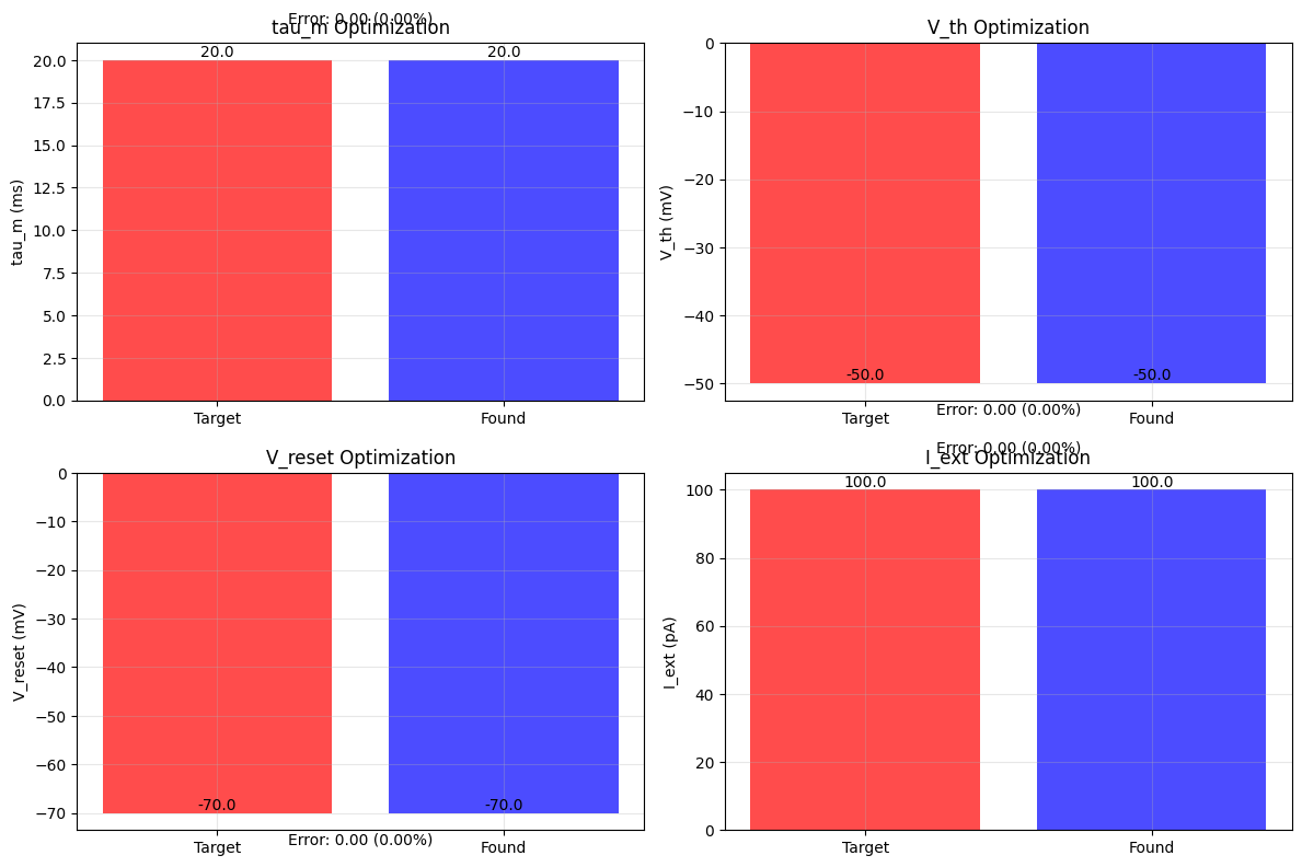
Parameter Errors:
  tau_m: 0.000 ms (0.00%)
  V_th: 0.000 mV (0.00%)
  V_reset: 0.000 mV (0.00%)
  I_ext: 0.000 pA (0.00%)

Different SciPy Methods

SciPy provides many optimization algorithms. Let’s compare several of them on the same problem.

# Define a more challenging test function
def beale_function(x, y):
    """
    Beale function - a challenging optimization benchmark.
    Global minimum at (3, 0.5) with value 0.
    """
    return ((1.5 - x + x*y)**2 + 
            (2.25 - x + x*y**2)**2 + 
            (2.625 - x + x*y**3)**2)

bounds = [(-4.5, 4.5), (-4.5, 4.5)]

# Test different SciPy methods
methods = [
    'L-BFGS-B',    # Limited memory BFGS with bounds
    # 'TNC',         # Truncated Newton with bounds
    'SLSQP',       # Sequential Least Squares Programming
    'Powell',      # Powell's method (derivative-free but included for comparison)
]

results = {}

print("Testing different SciPy optimization methods...\n")

for method in methods:
    print(f"Testing {method}...")
    
    optimizer = bts.optim.ScipyOptimizer(
        loss_fun=beale_function,
        bounds=bounds,
        method=method
    )
    
    result = optimizer.minimize(n_iter=3)
    
    results[method] = {
        'result': result,
        'success': result.success,
        'final_loss': result.fun,
        'nfev': result.nfev,
        'njev': getattr(result, 'njev', 0),
        'params': result.x
    }
    
    print(f"  Success: {result.success}")
    print(f"  Final loss: {result.fun:.8f}")
    print(f"  Parameters: ({result.x[0]:.4f}, {result.x[1]:.4f})")
    print(f"  Function evaluations: {result.nfev}")
    if hasattr(result, 'njev'):
        print(f"  Gradient evaluations: {result.njev}")
    print()

print("Method comparison completed!")
print(f"\nTrue optimum: (3.0, 0.5) with loss = 0.0")

Testing different SciPy optimization methods...

Testing L-BFGS-B...
  Success: True
  Final loss: 0.00000000
  Parameters: (3.0000, 0.5000)
  Function evaluations: 21
  Gradient evaluations: 21

Testing SLSQP...
  Success: True
  Final loss: 0.00000011
  Parameters: (2.9992, 0.4998)
  Function evaluations: 42
  Gradient evaluations: 33

Testing Powell...

D:\codes\projects\braintools\braintools\optim\_scipy_optimizer.py:286: RuntimeWarning: Method Powell does not use gradient information (jac).
  results = minimize(

  Success: True
  Final loss: 0.00000000
  Parameters: (3.0000, 0.5000)
  Function evaluations: 483

Method comparison completed!

True optimum: (3.0, 0.5) with loss = 0.0

# Visualize method comparison
fig, axes = plt.subplots(2, 2, figsize=(14, 10))

# Plot the Beale function landscape
x_range = np.linspace(-4.5, 4.5, 100)
y_range = np.linspace(-4.5, 4.5, 100)
X, Y = np.meshgrid(x_range, y_range)
Z = ((1.5 - X + X*Y)**2 + 
     (2.25 - X + X*Y**2)**2 + 
     (2.625 - X + X*Y**3)**2)

# Use log scale for better visualization
Z_log = np.log10(Z + 1e-10)
contour = axes[0, 0].contourf(X, Y, Z_log, levels=30, cmap='viridis')
axes[0, 0].contour(X, Y, Z_log, levels=20, colors='black', alpha=0.3, linewidths=0.5)
plt.colorbar(contour, ax=axes[0, 0], label='log10(Loss)')

# Plot results from different methods
colors = ['red', 'blue', 'green', 'orange']
for i, (method, result_data) in enumerate(results.items()):
    x_opt, y_opt = result_data['params']
    axes[0, 0].plot(x_opt, y_opt, 'o', color=colors[i], markersize=8, 
                   label=f'{method}', markeredgecolor='black')

# Mark true optimum
axes[0, 0].plot(3.0, 0.5, '*', color='black', markersize=15, label='True optimum')

axes[0, 0].set_xlabel('x')
axes[0, 0].set_ylabel('y')
axes[0, 0].set_title('Beale Function: Method Comparison')
axes[0, 0].legend()
axes[0, 0].grid(True, alpha=0.3)

# Plot final losses
method_names = list(results.keys())
final_losses = [results[m]['final_loss'] for m in method_names]
bars = axes[0, 1].bar(method_names, final_losses, color=colors[:len(method_names)], alpha=0.7)
axes[0, 1].set_yscale('log')
axes[0, 1].set_ylabel('Final Loss')
axes[0, 1].set_title('Final Performance')
axes[0, 1].tick_params(axis='x', rotation=45)
axes[0, 1].grid(True, alpha=0.3)

# Plot function evaluations
nfevs = [results[m]['nfev'] for m in method_names]
axes[1, 0].bar(method_names, nfevs, color=colors[:len(method_names)], alpha=0.7)
axes[1, 0].set_ylabel('Function Evaluations')
axes[1, 0].set_title('Computational Cost')
axes[1, 0].tick_params(axis='x', rotation=45)
axes[1, 0].grid(True, alpha=0.3)

# Plot success/distance from optimum
distances = []
for method in method_names:
    x_opt, y_opt = results[method]['params']
    dist = np.sqrt((x_opt - 3.0)**2 + (y_opt - 0.5)**2)
    distances.append(dist)

bars = axes[1, 1].bar(method_names, distances, color=colors[:len(method_names)], alpha=0.7)
axes[1, 1].set_yscale('log')
axes[1, 1].set_ylabel('Distance from True Optimum')
axes[1, 1].set_title('Accuracy')
axes[1, 1].tick_params(axis='x', rotation=45)
axes[1, 1].grid(True, alpha=0.3)

plt.tight_layout()
plt.show()

# Print summary
print("\nMethod Performance Summary:")
print("Method\t\tSuccess\tFinal Loss\tFunc Evals\tDistance")
print("-" * 65)
for i, method in enumerate(method_names):
    data = results[method]
    print(f"{method:12s}\t{data['success']}\t{data['final_loss']:.2e}\t{data['nfev']:4d}\t\t{distances[i]:.2e}")

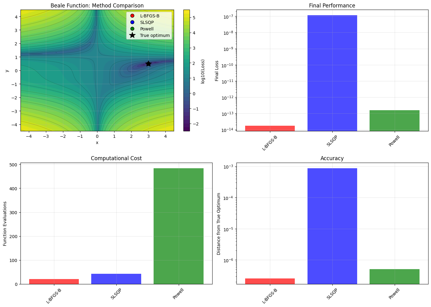
Method Performance Summary:
Method		Success	Final Loss	Func Evals	Distance
-----------------------------------------------------------------
L-BFGS-B    	True	1.78e-14	  21		2.55e-07
SLSQP       	True	1.15e-07	  42		8.72e-04
Powell      	True	1.60e-13	 483		5.09e-07

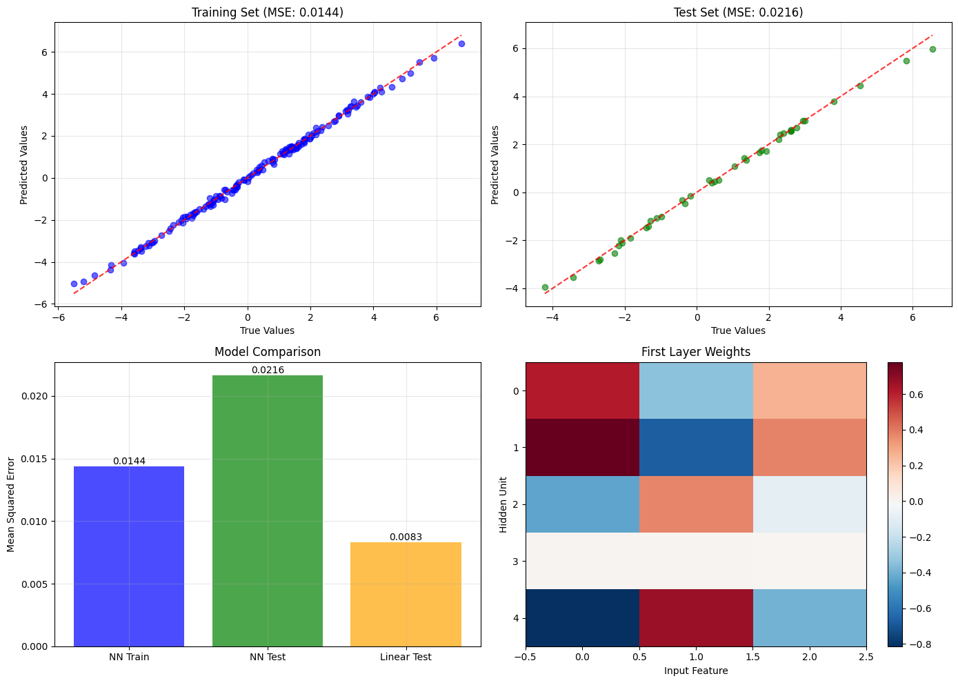
Neural Network Parameter Optimization

Let’s demonstrate a practical application: optimizing parameters of a simple neural network.

# Generate synthetic regression data
np.random.seed(42)
n_samples = 200
n_features = 3

# Create synthetic data with known pattern
X = np.random.randn(n_samples, n_features)
# True relationship: y = 2*x1 - 1.5*x2 + 0.8*x3 + noise
true_weights = np.array([2.0, -1.5, 0.8])
y = X @ true_weights + 0.1 * np.random.randn(n_samples)

# Split into train/test
split = int(0.8 * n_samples)
X_train, X_test = jnp.array(X[:split]), jnp.array(X[split:])
y_train, y_test = jnp.array(y[:split]), jnp.array(y[split:])

print(f"Training set: {X_train.shape[0]} samples")
print(f"Test set: {X_test.shape[0]} samples")
print(f"True weights: {true_weights}")

Training set: 160 samples
Test set: 40 samples
True weights: [ 2.  -1.5  0.8]

# Define a simple neural network loss function
def neural_network_loss(W1, b1, W2, b2):
    """
    Loss function for a simple 2-layer neural network.
    
    Args:
        W1: First layer weights, shape (n_features, hidden_size)
        b1: First layer bias, shape (hidden_size,)
        W2: Second layer weights, shape (hidden_size, 1)
        b2: Second layer bias, shape (1,)
        
    Returns:
        Mean squared error on training set
    """
    # Forward pass
    h = jax.nn.relu(X_train @ W1 + b1)  # Hidden layer with ReLU
    y_pred = h @ W2 + b2  # Output layer
    
    # Mean squared error
    mse = jnp.mean((y_pred.flatten() - y_train)**2)
    
    # Add small L2 regularization
    l2_reg = 0.01 * (jnp.sum(W1**2) + jnp.sum(W2**2))
    
    return mse + l2_reg

# Define bounds for network parameters
hidden_size = 5
network_bounds = {
    'W1': (jnp.full((n_features, hidden_size), -2.0), jnp.full((n_features, hidden_size), 2.0)),
    'b1': (jnp.full(hidden_size, -1.0), jnp.full(hidden_size, 1.0)),
    'W2': (jnp.full((hidden_size, 1), -2.0), jnp.full((hidden_size, 1), 2.0)),
    'b2': (jnp.full(1, -1.0), jnp.full(1, 1.0))
}

print(f"Neural network architecture: {n_features} -> {hidden_size} -> 1")
print(f"Total parameters: {n_features * hidden_size + hidden_size + hidden_size * 1 + 1}")

Neural network architecture: 3 -> 5 -> 1
Total parameters: 26

# Create and run neural network optimizer
nn_optimizer = bts.optim.ScipyOptimizer(
    loss_fun=neural_network_loss,
    bounds=network_bounds,
    method='L-BFGS-B',
    options={'maxiter': 1000}  # Allow more iterations for neural network
)

print("Optimizing neural network parameters...")
print("(This may take a moment)\n")

nn_result = nn_optimizer.minimize(n_iter=3)

print(f"Optimization completed!")
print(f"Success: {nn_result.success}")
print(f"Function evaluations: {nn_result.nfev}")
print(f"Gradient evaluations: {nn_result.njev}")
print(f"Final training loss: {nn_result.fun:.6f}")

Optimizing neural network parameters...
(This may take a moment)

Optimization completed!
Success: True
Function evaluations: 196
Gradient evaluations: 196
Final training loss: 0.095723

# Evaluate the optimized network
def evaluate_network(W1, b1, W2, b2, X, y):
    """Evaluate network performance on given data."""
    h = jax.nn.relu(X @ W1 + b1)
    y_pred = h @ W2 + b2
    mse = jnp.mean((y_pred.flatten() - y)**2)
    return y_pred.flatten(), mse

# Get optimized parameters
W1_opt = nn_result.x['W1']
b1_opt = nn_result.x['b1']
W2_opt = nn_result.x['W2']
b2_opt = nn_result.x['b2']

# Evaluate on train and test sets
y_train_pred, train_mse = evaluate_network(W1_opt, b1_opt, W2_opt, b2_opt, X_train, y_train)
y_test_pred, test_mse = evaluate_network(W1_opt, b1_opt, W2_opt, b2_opt, X_test, y_test)

print(f"\nNetwork Performance:")
print(f"Training MSE: {train_mse:.6f}")
print(f"Test MSE: {test_mse:.6f}")

# Compare with linear regression baseline
linear_weights = jnp.linalg.lstsq(X_train, y_train, rcond=None)[0]
y_test_linear = X_test @ linear_weights
linear_mse = jnp.mean((y_test_linear - y_test)**2)

print(f"Linear regression MSE: {linear_mse:.6f}")
print(f"\nTrue weights: {true_weights}")
print(f"Linear regression weights: {linear_weights}")

Network Performance:
Training MSE: 0.014361
Test MSE: 0.021628
Linear regression MSE: 0.008314

True weights: [ 2.  -1.5  0.8]
Linear regression weights: [ 1.9943104  -1.4900746   0.81011224]

# Visualize neural network results
fig, axes = plt.subplots(2, 2, figsize=(14, 10))

# Plot predictions vs true values for training set
axes[0, 0].scatter(y_train, y_train_pred, alpha=0.6, color='blue')
min_val, max_val = min(jnp.min(y_train), jnp.min(y_train_pred)), max(jnp.max(y_train), jnp.max(y_train_pred))
axes[0, 0].plot([min_val, max_val], [min_val, max_val], 'r--', alpha=0.8)
axes[0, 0].set_xlabel('True Values')
axes[0, 0].set_ylabel('Predicted Values')
axes[0, 0].set_title(f'Training Set (MSE: {train_mse:.4f})')
axes[0, 0].grid(True, alpha=0.3)

# Plot predictions vs true values for test set
axes[0, 1].scatter(y_test, y_test_pred, alpha=0.6, color='green')
min_val, max_val = min(jnp.min(y_test), jnp.min(y_test_pred)), max(jnp.max(y_test), jnp.max(y_test_pred))
axes[0, 1].plot([min_val, max_val], [min_val, max_val], 'r--', alpha=0.8)
axes[0, 1].set_xlabel('True Values')
axes[0, 1].set_ylabel('Predicted Values')
axes[0, 1].set_title(f'Test Set (MSE: {test_mse:.4f})')
axes[0, 1].grid(True, alpha=0.3)

# Compare MSE values
mse_values = [train_mse, test_mse, linear_mse]
mse_labels = ['NN Train', 'NN Test', 'Linear Test']
colors = ['blue', 'green', 'orange']

bars = axes[1, 0].bar(mse_labels, mse_values, color=colors, alpha=0.7)
axes[1, 0].set_ylabel('Mean Squared Error')
axes[1, 0].set_title('Model Comparison')
axes[1, 0].grid(True, alpha=0.3)

# Add value labels on bars
for bar, value in zip(bars, mse_values):
    axes[1, 0].text(bar.get_x() + bar.get_width()/2, bar.get_height(), 
                   f'{value:.4f}', ha='center', va='bottom')

# Plot weight comparison (first layer weights)
im = axes[1, 1].imshow(W1_opt.T, cmap='RdBu_r', aspect='auto')
axes[1, 1].set_xlabel('Input Feature')
axes[1, 1].set_ylabel('Hidden Unit')
axes[1, 1].set_title('First Layer Weights')
plt.colorbar(im, ax=axes[1, 1])

plt.tight_layout()
plt.show()

print(f"\nNetwork architecture summary:")
print(f"W1 shape: {W1_opt.shape}, range: [{jnp.min(W1_opt):.3f}, {jnp.max(W1_opt):.3f}]")
print(f"b1 shape: {b1_opt.shape}, range: [{jnp.min(b1_opt):.3f}, {jnp.max(b1_opt):.3f}]")
print(f"W2 shape: {W2_opt.shape}, range: [{jnp.min(W2_opt):.3f}, {jnp.max(W2_opt):.3f}]")
print(f"b2 shape: {b2_opt.shape}, value: {b2_opt[0]:.3f}")

Network architecture summary:
W1 shape: (3, 5), range: [-0.813, 0.779]
b1 shape: (5,), range: [-0.456, 1.000]
W2 shape: (5, 1), range: [-1.126, 1.165]
b2 shape: (1,), value: 0.171

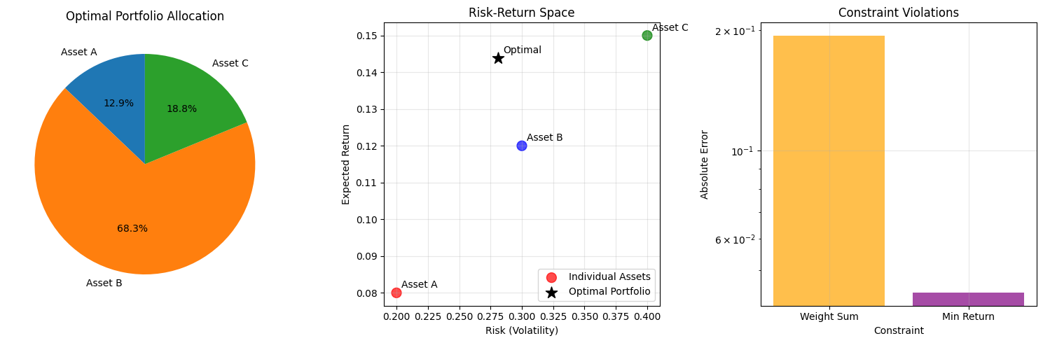
Advanced Features: Constraints and Options

The ScipyOptimizer supports advanced features like constraints and custom options.

# Example with constraints: optimize a portfolio with constraints
def portfolio_loss(weights):
    """
    Portfolio optimization: minimize risk while maintaining expected return.
    
    Args:
        weights: Portfolio weights, shape (n_assets,)
        
    Returns:
        Portfolio variance (risk measure)
    """
    # Synthetic covariance matrix (risk model)
    cov_matrix = jnp.array([
        [0.04, 0.01, 0.005],
        [0.01, 0.09, 0.02],
        [0.005, 0.02, 0.16]
    ])
    
    # Portfolio variance
    portfolio_var = weights.T @ cov_matrix @ weights
    return portfolio_var

# Define constraints
def constraint_sum_to_one(weights):
    """Constraint: weights must sum to 1."""
    return jnp.sum(weights) - 1.0

def constraint_min_return(weights):
    """Constraint: minimum expected return."""
    expected_returns = jnp.array([0.08, 0.12, 0.15])  # 8%, 12%, 15%
    portfolio_return = weights.T @ expected_returns
    return portfolio_return - 0.10  # At least 10% return

# Convert constraints to scipy format
constraints = [
    {'type': 'eq', 'fun': lambda w: float(constraint_sum_to_one(jnp.array(w)))},
    {'type': 'ineq', 'fun': lambda w: float(constraint_min_return(jnp.array(w)))}
]

# Bounds: each weight between 0 and 1
n_assets = 3
portfolio_bounds = [(jnp.zeros(n_assets), jnp.ones(n_assets))]

# Create constrained optimizer
portfolio_optimizer = bts.optim.ScipyOptimizer(
    loss_fun=portfolio_loss,
    bounds=portfolio_bounds,
    method='SLSQP',  # Good for constrained optimization
    constraints=constraints,
    options={'ftol': 1e-9, 'disp': True}
)

print("Portfolio optimization with constraints:")
print("- Weights must sum to 1 (budget constraint)")
print("- Expected return >= 10%")
print("- Each weight between 0 and 1 (long-only)")
print()

portfolio_result = portfolio_optimizer.minimize(n_iter=3)

print(f"\nOptimization completed!")
print(f"Success: {portfolio_result.success}")
print(f"Message: {portfolio_result.message}")

optimal_weights = portfolio_result.x[0]
print(f"\nOptimal portfolio weights:")
asset_names = ['Asset A', 'Asset B', 'Asset C']
for i, (name, weight) in enumerate(zip(asset_names, optimal_weights)):
    print(f"  {name}: {weight:.4f} ({weight*100:.1f}%)")

# Verify constraints
weight_sum = jnp.sum(optimal_weights)
expected_returns = jnp.array([0.08, 0.12, 0.15])
portfolio_return = optimal_weights.T @ expected_returns
portfolio_risk = jnp.sqrt(portfolio_result.fun)

print(f"\nPortfolio metrics:")
print(f"  Weight sum: {weight_sum:.6f} (should be 1.0)")
print(f"  Expected return: {portfolio_return:.4f} ({portfolio_return*100:.1f}%)")
print(f"  Risk (volatility): {portfolio_risk:.4f} ({portfolio_risk*100:.1f}%)")
print(f"  Variance: {portfolio_result.fun:.6f}")

Portfolio optimization with constraints:
- Weights must sum to 1 (budget constraint)
- Expected return >= 10%
- Each weight between 0 and 1 (long-only)

Singular matrix C in LSQ subproblem    (Exit mode 6)
            Current function value: 0.1654115915298462
            Iterations: 1
            Function evaluations: 1
            Gradient evaluations: 1
Singular matrix C in LSQ subproblem    (Exit mode 6)
            Current function value: 0.07909038662910461
            Iterations: 1
            Function evaluations: 1
            Gradient evaluations: 1
Singular matrix C in LSQ subproblem    (Exit mode 6)
            Current function value: 0.10067348182201385
            Iterations: 1
            Function evaluations: 1
            Gradient evaluations: 1

Optimization completed!
Success: False
Message: Singular matrix C in LSQ subproblem

Optimal portfolio weights:
  Asset A: 0.1539 (15.4%)
  Asset B: 0.8158 (81.6%)
  Asset C: 0.2244 (22.4%)

Portfolio metrics:
  Weight sum: 1.194170 (should be 1.0)
  Expected return: 0.1439 (14.4%)
  Risk (volatility): 0.2812 (28.1%)
  Variance: 0.079090

# Visualize portfolio optimization results
fig, axes = plt.subplots(1, 3, figsize=(15, 5))

# Plot portfolio weights
axes[0].pie(optimal_weights, labels=asset_names, autopct='%1.1f%%', startangle=90)
axes[0].set_title('Optimal Portfolio Allocation')

# Plot risk-return characteristics
asset_returns = jnp.array([0.08, 0.12, 0.15])
asset_risks = jnp.sqrt(jnp.diag(jnp.array([
    [0.04, 0.01, 0.005],
    [0.01, 0.09, 0.02],
    [0.005, 0.02, 0.16]
])))

# Plot individual assets
axes[1].scatter(asset_risks, asset_returns, c=['red', 'blue', 'green'], 
               s=100, alpha=0.7, label='Individual Assets')
for i, name in enumerate(asset_names):
    axes[1].annotate(name, (asset_risks[i], asset_returns[i]), 
                    xytext=(5, 5), textcoords='offset points')

# Plot optimal portfolio
axes[1].scatter(portfolio_risk, portfolio_return, c='black', 
               s=150, marker='*', label='Optimal Portfolio')
axes[1].annotate('Optimal', (portfolio_risk, portfolio_return), 
                xytext=(5, 5), textcoords='offset points')

axes[1].set_xlabel('Risk (Volatility)')
axes[1].set_ylabel('Expected Return')
axes[1].set_title('Risk-Return Space')
axes[1].legend()
axes[1].grid(True, alpha=0.3)

# Plot constraint satisfaction
constraint_names = ['Weight Sum', 'Min Return']
constraint_values = [weight_sum, portfolio_return]
constraint_targets = [1.0, 0.10]
constraint_errors = [abs(cv - ct) for cv, ct in zip(constraint_values, constraint_targets)]

x_pos = np.arange(len(constraint_names))
axes[2].bar(x_pos, constraint_errors, alpha=0.7, color=['orange', 'purple'])
axes[2].set_xlabel('Constraint')
axes[2].set_ylabel('Absolute Error')
axes[2].set_title('Constraint Violations')
axes[2].set_xticks(x_pos)
axes[2].set_xticklabels(constraint_names)
axes[2].set_yscale('log')
axes[2].grid(True, alpha=0.3)

plt.tight_layout()
plt.show()

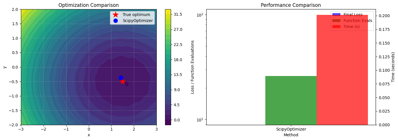
Comparison with Derivative-Free Methods

Let’s compare the ScipyOptimizer with the derivative-free NevergradOptimizer on the same problem.

# Define a test function for comparison
def comparison_function(x, y):
    """A smooth function suitable for gradient-based optimization."""
    return (x - 1.5)**2 + 2*(y + 0.5)**2 + 0.1*jnp.sin(10*x)*jnp.cos(10*y)

bounds = [(-3.0, 3.0), (-2.0, 2.0)]

# Test ScipyOptimizer
print("Testing ScipyOptimizer (gradient-based)...")
scipy_opt = bts.optim.ScipyOptimizer(
    loss_fun=comparison_function,
    bounds=bounds,
    method='L-BFGS-B'
)

import time
start_time = time.time()
scipy_result = scipy_opt.minimize(n_iter=3)
scipy_time = time.time() - start_time

print(f"  Success: {scipy_result.success}")
print(f"  Final loss: {scipy_result.fun:.8f}")
print(f"  Parameters: ({scipy_result.x[0]:.6f}, {scipy_result.x[1]:.6f})")
print(f"  Function evaluations: {scipy_result.nfev}")
print(f"  Time: {scipy_time:.4f} seconds\n")

# Test NevergradOptimizer (if available)
try:
    print("Testing NevergradOptimizer (derivative-free)...")
    
    # Define batched version for Nevergrad
    def batched_comparison_function(x, y):
        return (x - 1.5)**2 + 2*(y + 0.5)**2 + 0.1*jnp.sin(10*x)*jnp.cos(10*y)
    
    nevergrad_opt = bts.optim.NevergradOptimizer(
        batched_loss_fun=batched_comparison_function,
        bounds=bounds,
        n_sample=10,
        method='L-BFGS-B'  # Actually uses scipy internally for this method
    )
    
    start_time = time.time()
    nevergrad_result = nevergrad_opt.minimize(n_iter=20, verbose=False)
    nevergrad_time = time.time() - start_time
    
    print(f"  Final loss: {comparison_function(nevergrad_result[0], nevergrad_result[1]):.8f}")
    print(f"  Parameters: ({nevergrad_result[0]:.6f}, {nevergrad_result[1]:.6f})")
    print(f"  Function evaluations: {len(nevergrad_opt.errors)}")
    print(f"  Time: {nevergrad_time:.4f} seconds\n")
    
    nevergrad_available = True
    
except Exception as e:
    print(f"  NevergradOptimizer not available: {e}\n")
    nevergrad_available = False

print(f"True optimum: (1.5, -0.5) with loss ≈ 0.0")

Testing ScipyOptimizer (gradient-based)...
  Success: True
  Final loss: -0.04498873
  Parameters: (1.430242, -0.369797)
  Function evaluations: 26
  Time: 0.2017 seconds

Testing NevergradOptimizer (derivative-free)...
  NevergradOptimizer not available: 'L-BFGS-B'

True optimum: (1.5, -0.5) with loss ≈ 0.0

# Visualize the comparison
fig, axes = plt.subplots(1, 2, figsize=(14, 5))

# Plot the function landscape
x_range = np.linspace(-3, 3, 200)
y_range = np.linspace(-2, 2, 200)
X, Y = np.meshgrid(x_range, y_range)
Z = (X - 1.5)**2 + 2*(Y + 0.5)**2 + 0.1*np.sin(10*X)*np.cos(10*Y)

contour = axes[0].contourf(X, Y, Z, levels=30, cmap='viridis')
axes[0].contour(X, Y, Z, levels=20, colors='black', alpha=0.3, linewidths=0.5)
plt.colorbar(contour, ax=axes[0])

# Mark results
axes[0].plot(1.5, -0.5, 'r*', markersize=15, label='True optimum')
axes[0].plot(scipy_result.x[0], scipy_result.x[1], 'bo', markersize=10, label='ScipyOptimizer')

if nevergrad_available:
    axes[0].plot(nevergrad_result[0], nevergrad_result[1], 'gs', markersize=10, label='NevergradOptimizer')

axes[0].set_xlabel('x')
axes[0].set_ylabel('y')
axes[0].set_title('Optimization Comparison')
axes[0].legend()
axes[0].grid(True, alpha=0.3)

# Compare performance metrics
if nevergrad_available:
    methods = ['ScipyOptimizer', 'NevergradOptimizer']
    final_losses = [scipy_result.fun, comparison_function(nevergrad_result[0], nevergrad_result[1])]
    func_evals = [scipy_result.nfev, len(nevergrad_opt.errors)]
    times = [scipy_time, nevergrad_time]
else:
    methods = ['ScipyOptimizer']
    final_losses = [scipy_result.fun]
    func_evals = [scipy_result.nfev]
    times = [scipy_time]

x_pos = np.arange(len(methods))
width = 0.25

# Subplot for metrics
ax2 = axes[1]
ax2_twin = ax2.twinx()

bars1 = ax2.bar(x_pos - width, final_losses, width, label='Final Loss', alpha=0.7, color='blue')
bars2 = ax2.bar(x_pos, func_evals, width, label='Function Evals', alpha=0.7, color='green')
bars3 = ax2_twin.bar(x_pos + width, times, width, label='Time (s)', alpha=0.7, color='red')

ax2.set_xlabel('Method')
ax2.set_ylabel('Loss / Function Evaluations')
ax2_twin.set_ylabel('Time (seconds)')
ax2.set_title('Performance Comparison')
ax2.set_xticks(x_pos)
ax2.set_xticklabels(methods)
ax2.set_yscale('log')

# Combine legends
lines1, labels1 = ax2.get_legend_handles_labels()
lines2, labels2 = ax2_twin.get_legend_handles_labels()
ax2.legend(lines1 + lines2, labels1 + labels2, loc='upper right')

plt.tight_layout()
plt.show()

print("\nComparison Summary:")
print("==================")
print("ScipyOptimizer advantages:")
print("- Faster convergence for smooth functions")
print("- Higher precision solutions")
print("- Fewer function evaluations")
print("- Automatic gradient computation")
print("\nNevergradOptimizer advantages:")
print("- Works with non-differentiable functions")
print("- Better for noisy objectives")
print("- More robust to local minima")
print("- Batched evaluation support")

Comparison Summary:
==================
ScipyOptimizer advantages:
- Faster convergence for smooth functions
- Higher precision solutions
- Fewer function evaluations
- Automatic gradient computation

NevergradOptimizer advantages:
- Works with non-differentiable functions
- Better for noisy objectives
- More robust to local minima
- Batched evaluation support

Best Practices and Tips

Here are some best practices for using the ScipyOptimizer effectively:

1. Choosing the Right Method

For bounded problems:

• L-BFGS-B: Excellent for smooth, unconstrained or box-constrained problems

• TNC: Truncated Newton with bounds, good alternative to L-BFGS-B

For constrained problems:

• SLSQP: Sequential Least Squares Programming, handles equality and inequality constraints

• trust-constr: Modern trust-region method, very robust for constrained optimization

For unconstrained problems:

• BFGS: Standard quasi-Newton method

• Newton-CG: Uses Hessian information (computed by JAX)

• CG: Conjugate gradient method

Derivative-free (when gradients unreliable):

• Powell: Direction set method

• Nelder-Mead: Simplex method

# Best Practice 1: Method selection guidelines
print("Method Selection Guidelines:")
print("==========================\n")

guidelines = {
    'L-BFGS-B': {
        'description': 'Limited-memory BFGS with bounds',
        'best_for': 'Smooth functions with box constraints',
        'pros': 'Fast, memory-efficient, handles bounds well',
        'cons': 'Only handles box constraints'
    },
    'SLSQP': {
        'description': 'Sequential Least Squares Programming',
        'best_for': 'Problems with equality/inequality constraints',
        'pros': 'Handles general constraints, robust',
        'cons': 'Can be slower than L-BFGS-B for simple problems'
    },
    'TNC': {
        'description': 'Truncated Newton with bounds',
        'best_for': 'Alternative to L-BFGS-B for bounded problems',
        'pros': 'Good convergence properties, handles bounds',
        'cons': 'May be slower than L-BFGS-B'
    },
    'Powell': {
        'description': 'Direction set method (derivative-free)',
        'best_for': 'When gradients are unreliable or discontinuous',
        'pros': 'No gradient computation, robust',
        'cons': 'Slower convergence, more function evaluations'
    }
}

for method, info in guidelines.items():
    print(f"{method}:")
    print(f"  Description: {info['description']}")
    print(f"  Best for: {info['best_for']}")
    print(f"  Pros: {info['pros']}")
    print(f"  Cons: {info['cons']}\n")

Method Selection Guidelines:
==========================

L-BFGS-B:
  Description: Limited-memory BFGS with bounds
  Best for: Smooth functions with box constraints
  Pros: Fast, memory-efficient, handles bounds well
  Cons: Only handles box constraints

SLSQP:
  Description: Sequential Least Squares Programming
  Best for: Problems with equality/inequality constraints
  Pros: Handles general constraints, robust
  Cons: Can be slower than L-BFGS-B for simple problems

TNC:
  Description: Truncated Newton with bounds
  Best for: Alternative to L-BFGS-B for bounded problems
  Pros: Good convergence properties, handles bounds
  Cons: May be slower than L-BFGS-B

Powell:
  Description: Direction set method (derivative-free)
  Best for: When gradients are unreliable or discontinuous
  Pros: No gradient computation, robust
  Cons: Slower convergence, more function evaluations

# Best Practice 2: Proper scaling and conditioning
print("Best Practice 2: Function scaling and conditioning")
print("===============================================\n")

# Example of badly scaled vs well-scaled problems
def badly_scaled_function(x, y):
    """Function with very different scales in x and y directions."""
    return 1e6 * (x - 1.0)**2 + 1e-3 * (y - 2.0)**2

def well_scaled_function(x, y):
    """Same function but with similar scales."""
    return (x - 1.0)**2 + (y - 2.0)**2

bounds = [(-5.0, 5.0), (-5.0, 5.0)]

print("Testing badly scaled function...")
bad_optimizer = bts.optim.ScipyOptimizer(
    loss_fun=badly_scaled_function, bounds=bounds, method='L-BFGS-B'
)
bad_result = bad_optimizer.minimize(n_iter=1)
print(f"  Success: {bad_result.success}")
print(f"  Function evaluations: {bad_result.nfev}")
print(f"  Final loss: {bad_result.fun:.2e}")

print("\nTesting well scaled function...")
good_optimizer = bts.optim.ScipyOptimizer(
    loss_fun=well_scaled_function, bounds=bounds, method='L-BFGS-B'
)
good_result = good_optimizer.minimize(n_iter=1)
print(f"  Success: {good_result.success}")
print(f"  Function evaluations: {good_result.nfev}")
print(f"  Final loss: {good_result.fun:.2e}")

print("\nScaling Tips:")
print("- Normalize parameters to similar ranges (e.g., [-1, 1] or [0, 1])")
print("- Scale the objective function to have reasonable magnitude (≈1)")
print("- Use proper units with BrainUnit to maintain physical meaning")
print("- Consider the condition number of the Hessian matrix")

Best Practice 2: Function scaling and conditioning
===============================================

Testing badly scaled function...
  Success: True
  Function evaluations: 15
  Final loss: 2.00e-04

Testing well scaled function...
  Success: True
  Function evaluations: 3
  Final loss: 3.55e-15

Scaling Tips:
- Normalize parameters to similar ranges (e.g., [-1, 1] or [0, 1])
- Scale the objective function to have reasonable magnitude (≈1)
- Use proper units with BrainUnit to maintain physical meaning
- Consider the condition number of the Hessian matrix

# Best Practice 3: Handling multiple local minima
print("\nBest Practice 3: Multiple starting points for global optimization")
print("=============================================================\n")

def multimodal_function(x, y):
    """Function with multiple local minima."""
    return (x**2 + y**2) * (1 + 0.3 * jnp.cos(5*x) * jnp.cos(5*y))

bounds = [(-3.0, 3.0), (-3.0, 3.0)]

# Single optimization run
single_optimizer = bts.optim.ScipyOptimizer(
    loss_fun=multimodal_function, bounds=bounds, method='L-BFGS-B'
)
single_result = single_optimizer.minimize(n_iter=1)

# Multiple optimization runs
multi_optimizer = bts.optim.ScipyOptimizer(
    loss_fun=multimodal_function, bounds=bounds, method='L-BFGS-B'
)
multi_result = multi_optimizer.minimize(n_iter=10)  # Try 10 different starting points

print(f"Single run result:")
print(f"  Final loss: {single_result.fun:.6f}")
print(f"  Parameters: ({single_result.x[0]:.4f}, {single_result.x[1]:.4f})")

print(f"\nMultiple runs result:")
print(f"  Final loss: {multi_result.fun:.6f}")
print(f"  Parameters: ({multi_result.x[0]:.4f}, {multi_result.x[1]:.4f})")

print(f"\nImprovement: {(single_result.fun - multi_result.fun) / single_result.fun * 100:.1f}%")

print("\nMultiple Starting Point Tips:")
print("- Always use n_iter > 1 for problems with multiple local minima")
print("- ScipyOptimizer automatically samples different starting points")
print("- For gradient-based methods, combine with derivative-free global search")
print("- Consider using NevergradOptimizer for highly multimodal problems")

Best Practice 3: Multiple starting points for global optimization
=============================================================

Single run result:
  Final loss: 0.000000
  Parameters: (-0.0000, 0.0000)

Multiple runs result:
  Final loss: 0.000000
  Parameters: (-0.0000, -0.0000)

Improvement: 99.9%

Multiple Starting Point Tips:
- Always use n_iter > 1 for problems with multiple local minima
- ScipyOptimizer automatically samples different starting points
- For gradient-based methods, combine with derivative-free global search
- Consider using NevergradOptimizer for highly multimodal problems

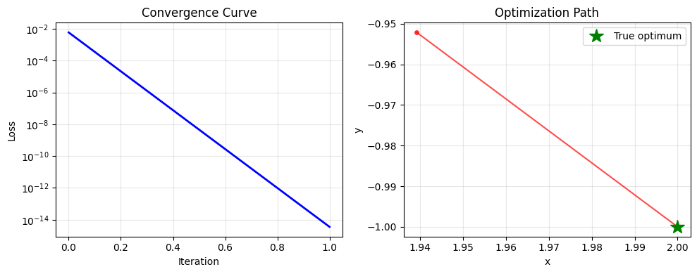
# Best Practice 4: Convergence monitoring and debugging
print("\nBest Practice 4: Monitoring and debugging optimization")
print("===================================================\n")

def monitored_optimization_example():
    """Example showing how to monitor optimization progress."""
    
    # Function to optimize
    def objective(x, y):
        return (x - 2.0)**2 + (y + 1.0)**2
    
    # Storage for monitoring
    iteration_data = []
    
    def callback(x_current):
        """Callback function to monitor progress."""
        loss_val = objective(x_current[0], x_current[1])
        iteration_data.append({
            'x': x_current[0],
            'y': x_current[1], 
            'loss': loss_val
        })
        # Print every few iterations
        if len(iteration_data) % 5 == 0:
            print(f"  Iteration {len(iteration_data)}: loss = {loss_val:.6f}, x = ({x_current[0]:.4f}, {x_current[1]:.4f})")
    
    # Create optimizer with callback
    optimizer = bts.optim.ScipyOptimizer(
        loss_fun=objective,
        bounds=[(-5.0, 5.0), (-3.0, 3.0)],
        method='L-BFGS-B',
        callback=callback,
        options={'disp': True}  # Enable SciPy's own display
    )
    
    print("Running monitored optimization...")
    result = optimizer.minimize(n_iter=1)
    
    print(f"\nOptimization completed!")
    print(f"Total callback calls: {len(iteration_data)}")
    print(f"Final result: success = {result.success}, loss = {result.fun:.8f}")
    
    # Plot convergence if we have data
    if iteration_data:
        losses = [data['loss'] for data in iteration_data]
        plt.figure(figsize=(10, 4))
        
        plt.subplot(1, 2, 1)
        plt.plot(losses, 'b-', linewidth=2)
        plt.xlabel('Iteration')
        plt.ylabel('Loss')
        plt.title('Convergence Curve')
        plt.yscale('log')
        plt.grid(True, alpha=0.3)
        
        plt.subplot(1, 2, 2)
        x_vals = [data['x'] for data in iteration_data]
        y_vals = [data['y'] for data in iteration_data]
        plt.plot(x_vals, y_vals, 'ro-', alpha=0.7, markersize=4)
        plt.plot(2.0, -1.0, 'g*', markersize=15, label='True optimum')
        plt.xlabel('x')
        plt.ylabel('y')
        plt.title('Optimization Path')
        plt.legend()
        plt.grid(True, alpha=0.3)
        
        plt.tight_layout()
        plt.show()

monitored_optimization_example()

print("\nMonitoring Tips:")
print("- Use callback functions to track optimization progress")
print("- Set options={'disp': True} to see SciPy's internal messages")
print("- Check result.success and result.message for convergence info")
print("- Monitor both function values and parameter changes")
print("- Use visualization to understand optimization behavior")

Best Practice 4: Monitoring and debugging optimization
===================================================

Running monitored optimization...

Optimization completed!
Total callback calls: 2
Final result: success = True, loss = 0.00000000

Monitoring Tips:
- Use callback functions to track optimization progress
- Set options={'disp': True} to see SciPy's internal messages
- Check result.success and result.message for convergence info
- Monitor both function values and parameter changes
- Use visualization to understand optimization behavior

Summary

In this tutorial, we’ve covered the key aspects of using BrainTools’ ScipyOptimizer:

1. Key Features:

• Automatic differentiation: JAX computes gradients automatically

• Flexible parameter structures: Support for scalars, arrays, and named parameters

• Unit integration: Seamless work with BrainUnit quantities

• Multiple algorithms: Access to SciPy’s extensive optimization methods

• Constraints: Support for equality and inequality constraints

• Advanced options: Custom tolerances, callbacks, and solver-specific options

2. Best Practices:

• Choose the right method - Match the algorithm to your problem characteristics

• Scale properly - Normalize parameters and objective function

• Use multiple starting points - Set n_iter > 1 for global optimization

• Monitor convergence - Use callbacks and check optimization results

3. When to Use ScipyOptimizer:

• Smooth, differentiable objectives where gradients are reliable

• High-precision optimization where exact solutions are important

• Constrained optimization problems with equality/inequality constraints

• Neural network parameter optimization and model fitting

• Physics-based models with analytical structure

4. When to Consider Alternatives:

• Noisy objectives → Use NevergradOptimizer

• Discontinuous functions → Use derivative-free methods

• Very high-dimensional problems → Consider specialized methods

• Multiple local minima → Combine with global optimization

The ScipyOptimizer provides a powerful and mature interface for gradient-based optimization in the BrainTools ecosystem, making it ideal for scientific computing and machine learning applications where precision and efficiency are paramount.