

Classification Losses#
braintools.metric provides the standard classification losses as pure JAX functions, so they work under jax.jit, jax.grad, and jax.vmap. They follow the same conventions as optax: inputs are logits (unnormalized scores), and the result is one loss value per example, which you reduce yourself (usually with .mean()).
Function |
Targets |
Use for |
|---|---|---|
|
0/1 (or probabilities), same shape as logits |
binary and multi-label problems |
|
one-hot or probability vectors |
single-label multiclass with soft targets |
|
class indices |
single-label multiclass |
|
0/1 |
binary / multi-label with many easy examples |
|
one-hot |
label smoothing before softmax CE |
|
class index |
when you already have log-probabilities |
|
±1 |
margin-based binary classifiers |
|
class indices |
margin-based multiclass |
|
one-hot |
PolyLoss (cross-entropy plus a polynomial term) |
|
probability vectors |
matching distributions |
Every function in the table was checked against its optax counterpart; the first cell below repeats that check.
1. Setup#
import jax
import jax.numpy as jnp
import matplotlib.pyplot as plt
import numpy as np
import optax

import braintools.metric as bm

key = jax.random.PRNGKey(0)
logits = jax.random.normal(key, (8, 4))
int_labels = jnp.arange(8) % 4
one_hot = jax.nn.one_hot(int_labels, 4)
binary = (jax.random.uniform(jax.random.PRNGKey(1), (8, 4)) < 0.5).astype(jnp.float32)

pairs = {
    "sigmoid_binary_cross_entropy": (bm.sigmoid_binary_cross_entropy(logits, binary), optax.sigmoid_binary_cross_entropy(logits, binary)),
    "softmax_cross_entropy": (bm.softmax_cross_entropy(logits, one_hot), optax.softmax_cross_entropy(logits, one_hot)),
    "..._with_integer_labels": (bm.softmax_cross_entropy_with_integer_labels(logits, int_labels),
                                optax.softmax_cross_entropy_with_integer_labels(logits, int_labels)),
    "sigmoid_focal_loss": (bm.sigmoid_focal_loss(logits, binary, alpha=0.25, gamma=2.0),
                           optax.sigmoid_focal_loss(logits, binary, alpha=0.25, gamma=2.0)),
    "smooth_labels": (bm.smooth_labels(one_hot, 0.1), optax.smooth_labels(one_hot, 0.1)),
    "hinge_loss": (bm.hinge_loss(logits, 2 * binary - 1), optax.hinge_loss(logits, 2 * binary - 1)),
}
for name, (ours, ref) in pairs.items():
    print(f"{name:30s} max |difference| from optax: {float(jnp.max(jnp.abs(ours - ref))):.1e}")
sigmoid_binary_cross_entropy   max |difference| from optax: 0.0e+00
softmax_cross_entropy          max |difference| from optax: 0.0e+00
..._with_integer_labels        max |difference| from optax: 1.2e-07
sigmoid_focal_loss             max |difference| from optax: 6.0e-08
smooth_labels                  max |difference| from optax: 0.0e+00
hinge_loss                     max |difference| from optax: 0.0e+00
2. Binary and Multi-Label: Sigmoid Cross-Entropy#
Each output is an independent yes/no decision:
It is computed from the logit \(z\) directly in a numerically stable form, so never apply sigmoid yourself first. Labels may be soft (probabilities).
z = jnp.array([4.0, -4.0, 0.0, 4.0])
y = jnp.array([1.0, 0.0, 1.0, 0.0])
print("per-element loss:", bm.sigmoid_binary_cross_entropy(z, y))
print("by hand:         ", -y * jnp.log(jax.nn.sigmoid(z)) - (1 - y) * jnp.log(1 - jax.nn.sigmoid(z)))
print("extreme logits stay finite:", bm.sigmoid_binary_cross_entropy(jnp.array([200.0]), jnp.array([0.0])))
per-element loss: [0.01814993 0.01814993 0.6931472 4.01815 ]
by hand:          [0.01814996 0.01814996 0.6931472  4.0181484 ]
extreme logits stay finite: [200.]
3. Multiclass: Softmax Cross-Entropy#
When exactly one class is correct, use softmax_cross_entropy_with_integer_labels with class indices; softmax_cross_entropy takes a probability vector per example (one-hot or soft). Both return \(-\sum_c y_c \log \operatorname{softmax}(z)_c\), so they agree for one-hot targets. nll_loss is the same quantity when you already hold log-probabilities.
z = jnp.array([[2.0, 1.0, 0.1]])
print("integer labels:", bm.softmax_cross_entropy_with_integer_labels(z, jnp.array([0])))
print("one-hot labels:", bm.softmax_cross_entropy(z, jnp.array([[1.0, 0.0, 0.0]])))
print("nll_loss:      ", bm.nll_loss(jax.nn.log_softmax(z[0]), 0))
print("soft target:   ", bm.softmax_cross_entropy(z, jnp.array([[0.7, 0.2, 0.1]])))
integer labels: [0.41702995]
one-hot labels: [0.41702995]
nll_loss:       0.41702995
soft target:    [0.8070299]
4. Focal Loss#
The focal loss multiplies the cross-entropy by \((1 - p_t)^\gamma\), where \(p_t\) is the probability the model assigns to the correct label. Well-classified examples (\(p_t \to 1\)) are down-weighted, so training concentrates on hard ones; \(\gamma = 0\) recovers the cross-entropy. alpha is an extra weight on the positive class (\(\alpha\) for positives, \(1 - \alpha\) for negatives); alpha=None disables it. In the original detector setting (Lin et al., 2017) the best value was \(\alpha = 0.25\) even though positives were rare, because \(\gamma\) already down-weights the many easy negatives, so treat alpha as a hyperparameter rather than the class frequency.
p_t = np.linspace(0.01, 0.99, 200)
logit_for_positive = np.log(p_t / (1 - p_t))  # label 1, so p_t = sigmoid(logit)
fig, ax = plt.subplots(figsize=(6, 3.5))
for gamma in [0.0, 1.0, 2.0, 5.0]:
    loss = bm.sigmoid_focal_loss(jnp.asarray(logit_for_positive), jnp.ones(200), alpha=None, gamma=gamma)
    ax.plot(p_t, loss, label=f"gamma = {gamma}")
ax.set_xlabel("probability of the correct label $p_t$")
ax.set_ylabel("loss")
ax.set_yscale("log")
ax.legend()
plt.show()

easy, hard = jnp.array([3.0]), jnp.array([-1.0])  # logits for a positive example
for g in [0.0, 2.0]:
    ratio = bm.sigmoid_focal_loss(hard, jnp.ones(1), gamma=g) / bm.sigmoid_focal_loss(easy, jnp.ones(1), gamma=g)
    print(f"gamma={g}: hard/easy loss ratio = {float(ratio[0]):.0f}")
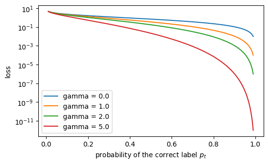
gamma=0.0: hard/easy loss ratio = 27
gamma=2.0: hard/easy loss ratio = 6422
5. Label Smoothing#
smooth_labels(labels, alpha) returns \((1 - \alpha)\,y + \alpha / C\) for \(C\) classes. Training against smoothed targets keeps the model from driving logits to infinity: the optimal logit gap becomes finite.
y = jnp.array([[1.0, 0.0, 0.0]])
print("smoothed:", bm.smooth_labels(y, alpha=0.1), "(0.9 + 0.1/3, 0.1/3, 0.1/3)")

gaps = jnp.linspace(0, 12, 200)
z = jnp.stack([gaps, jnp.zeros_like(gaps), jnp.zeros_like(gaps)], axis=1)
hard = bm.softmax_cross_entropy(z, jnp.repeat(y, 200, axis=0))
soft = bm.softmax_cross_entropy(z, jnp.repeat(bm.smooth_labels(y, 0.1), 200, axis=0))
print(f"loss keeps falling with a hard target; with smoothing the minimum is at gap {float(gaps[jnp.argmin(soft)]):.2f} "
      f"(theory: log((1 - a + a/C) / (a/C)) = {np.log((0.9 + 0.1 / 3) / (0.1 / 3)):.2f})")
smoothed: [[0.93333334 0.03333334 0.03333334]] (0.9 + 0.1/3, 0.1/3, 0.1/3)
loss keeps falling with a hard target; with smoothing the minimum is at gap 3.32 (theory: log((1 - a + a/C) / (a/C)) = 3.33)
6. Using a Loss for Training#
Because the losses are differentiable JAX functions, they plug straight into jax.grad. Here is a minimal logistic-regression fit with plain gradient descent.
kx, kw = jax.random.split(jax.random.PRNGKey(2))
X = jax.random.normal(kx, (400, 2))
true_w = jnp.array([2.0, -1.0])
y = (X @ true_w + 0.3 * jax.random.normal(kw, (400,)) > 0).astype(jnp.float32)


def loss_fn(params):
    logits = X @ params["w"] + params["b"]
    return bm.sigmoid_binary_cross_entropy(logits, y).mean()


params = {"w": jnp.zeros(2), "b": jnp.zeros(())}
grad_fn = jax.jit(jax.value_and_grad(loss_fn))
for step in range(300):
    loss, grads = grad_fn(params)
    params = jax.tree.map(lambda p, g: p - 0.5 * g, params, grads)

accuracy = jnp.mean(((X @ params["w"] + params["b"]) > 0) == (y > 0))
direction = params["w"] / jnp.linalg.norm(params["w"])
print(f"final loss {float(loss):.3f}, accuracy {float(accuracy):.3f}, learned direction {direction} "
      f"(true {true_w / jnp.linalg.norm(true_w)})")
final loss 0.128, accuracy 0.965, learned direction [ 0.90056664 -0.43471798] (true [ 0.8944272 -0.4472136])
Summary#
Pass logits, not probabilities; the losses apply the sigmoid/softmax internally in a stable way.
Multi-label:
sigmoid_binary_cross_entropy. Single-label:softmax_cross_entropy_with_integer_labels(indices) orsoftmax_cross_entropy(probability targets).Focal loss down-weights easy examples through
gamma;alphaweights positives versus negatives.smooth_labelsgives finite optimal logits. Losses are per example: reduce with.mean()before differentiating.