
Tutorial 3: Distance-Dependent Connectivity Patterns#
![]()
This tutorial explores distance-dependent connectivity patterns that are fundamental to spatial neural networks. In biological neural systems, connection probability and strength often depend on the physical distance between neurons.
Topics Covered#
Distance profiles for spatial neural connectivity
Basic profiles: Gaussian, Exponential, PowerLaw, Linear, Step
Advanced profiles: Sigmoid, DoG, Logistic, Bimodal, MexicanHat
Profile composition: arithmetic operations, clipping, transformations
Pipe operator for functional composition
Real-world neuroscience applications
Installation and Setup#
# Install braintools if needed
# !pip install braintools brainunit matplotlib numpy scipy
import numpy as np
import matplotlib.pyplot as plt
from matplotlib.gridspec import GridSpec
import brainunit as u
from braintools import init

# Set random seed for reproducibility
np.random.seed(42)

# Configure matplotlib
plt.rcParams['figure.figsize'] = (12, 4)
plt.rcParams['font.size'] = 10
1. Introduction to Distance-Dependent Connectivity#
Biological Motivation#
In the brain, neurons are spatially organized, and their connectivity follows specific patterns:
Local connectivity: Neurons close together are more likely to connect
Distance decay: Connection probability decreases with distance
Lateral inhibition: Nearby neurons may inhibit slightly distant ones
Long-range connections: Some neurons connect across large distances
Distance Profiles#
A distance profile defines how connection properties vary with spatial distance:
probability = profile.probability(distances)
weight_scaling = profile.weight_scaling(distances)
Key Concepts#
Connection probability: Likelihood of forming a connection
Weight scaling: Strength modulation based on distance
Spatial units: Using physical distances (μm, mm, etc.)
Profile composition: Combining multiple patterns
# Helper function to visualize profiles
def visualize_profile(profile, max_distance=200, title="Distance Profile", unit=u.um):
    """
    Visualize a distance profile.
    """
    distances = np.linspace(0, max_distance, 500) * unit
    probabilities = profile.probability(distances)
    weights = profile.weight_scaling(distances)

    fig, axes = plt.subplots(1, 2, figsize=(12, 4))

    # Probability
    axes[0].plot(distances.mantissa, probabilities, linewidth=2)
    axes[0].fill_between(distances.mantissa, probabilities, alpha=0.3)
    axes[0].set_xlabel(f'Distance ({unit})')
    axes[0].set_ylabel('Connection Probability')
    axes[0].set_title(f'{title} - Probability')
    axes[0].grid(alpha=0.3)
    axes[0].set_ylim([0, 1.1])

    # Weight scaling
    axes[1].plot(distances.mantissa, weights, linewidth=2, color='orange')
    axes[1].fill_between(distances.mantissa, weights, alpha=0.3, color='orange')
    axes[1].set_xlabel(f'Distance ({unit})')
    axes[1].set_ylabel('Weight Scaling Factor')
    axes[1].set_title(f'{title} - Weight Scaling')
    axes[1].grid(alpha=0.3)

    plt.tight_layout()
    plt.show()

    return distances, probabilities, weights
2. Basic Distance Profiles#
2.1 Gaussian Profile#
The Gaussian profile creates bell-shaped connectivity with peak at distance 0:
Parameters:
sigma: Standard deviation (controls spread)max_distance: Optional cutoff distance
Use cases:
Local excitatory connections
Smooth distance decay
Cortical columns
# Create Gaussian profile
gaussian = init.GaussianProfile(
    sigma=50.0 * u.um,
    max_distance=200.0 * u.um
)

distances, probs, weights = visualize_profile(gaussian, title="Gaussian Profile")

print(f"Gaussian Profile Properties:")
print(f"  Probability at 0 μm: {probs[0]:.3f}")
print(f"  Probability at 50 μm (1σ): {probs[250]:.3f}")
print(f"  Half-width at half-max: ~{50 * np.sqrt(2 * np.log(2)):.1f} μm")
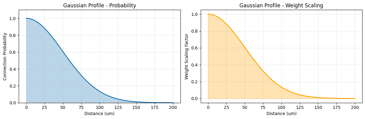
Gaussian Profile Properties:
  Probability at 0 μm: 1.000
  Probability at 50 μm (1σ): 0.134
  Half-width at half-max: ~58.9 μm
Effect of Sigma Parameter#
# Compare different sigma values
sigmas = [20.0, 50.0, 100.0]
colors = ['red', 'blue', 'green']

fig, ax = plt.subplots(1, 1, figsize=(10, 5))

distances = np.linspace(0, 200, 500) * u.um

for sigma, color in zip(sigmas, colors):
    profile = init.GaussianProfile(sigma=sigma * u.um)
    probs = profile.probability(distances)
    ax.plot(distances.mantissa, probs, linewidth=2, label=f'σ = {sigma} μm', color=color)
    ax.fill_between(distances.mantissa, probs, alpha=0.2, color=color)

ax.set_xlabel('Distance (μm)', fontsize=12)
ax.set_ylabel('Connection Probability', fontsize=12)
ax.set_title('Gaussian Profile: Effect of Sigma', fontsize=14)
ax.legend(fontsize=11)
ax.grid(alpha=0.3)

plt.tight_layout()
plt.show()

print("💡 Larger sigma → broader connectivity")
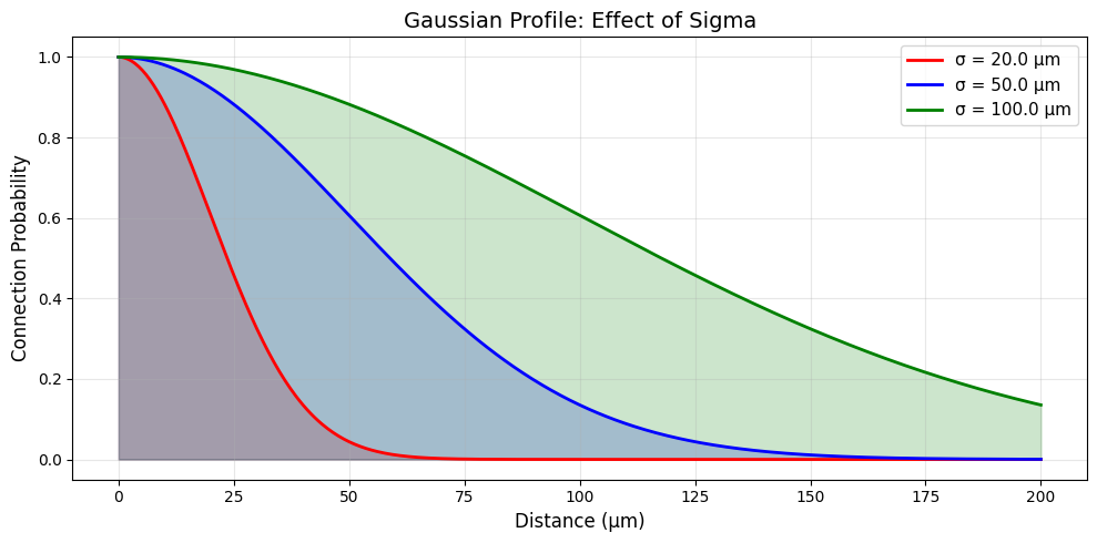
💡 Larger sigma → broader connectivity
2.2 Exponential Profile#
The Exponential profile creates monotonic decay:
Parameters:
decay_constant(λ): Distance constant for decaymax_distance: Optional cutoff
Use cases:
Long-range connections
Axonal arbor patterns
Distance-dependent decay
# Create Exponential profile
exponential = init.ExponentialProfile(
    decay_constant=75.0 * u.um,
    max_distance=300.0 * u.um
)

visualize_profile(exponential, max_distance=300, title="Exponential Profile")

print(f"\nExponential Profile Properties:")
print(f"  Probability at 0: 1.000")
print(f"  Probability at λ (75 μm): {np.exp(-1):.3f} ≈ 0.368")
print(f"  Probability at 2λ (150 μm): {np.exp(-2):.3f} ≈ 0.135")
print(f"  Half-distance: {75 * np.log(2):.1f} μm")
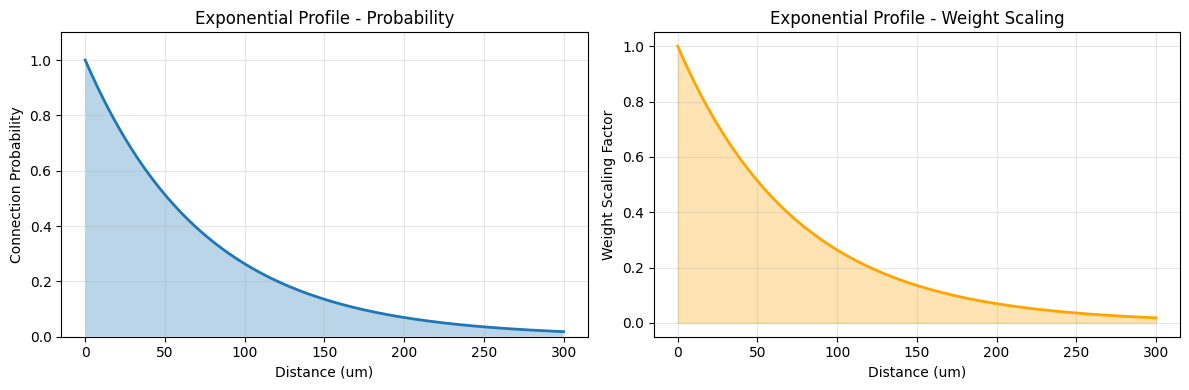
Exponential Profile Properties:
  Probability at 0: 1.000
  Probability at λ (75 μm): 0.368 ≈ 0.368
  Probability at 2λ (150 μm): 0.135 ≈ 0.135
  Half-distance: 52.0 μm
Gaussian vs Exponential#
# Compare Gaussian and Exponential
fig, axes = plt.subplots(1, 2, figsize=(14, 5))

distances = np.linspace(0, 200, 500) * u.um

gaussian_prof = init.GaussianProfile(sigma=50.0 * u.um)
exponential_prof = init.ExponentialProfile(decay_constant=50.0 * u.um)

gauss_prob = gaussian_prof.probability(distances)
exp_prob = exponential_prof.probability(distances)

# Linear scale
axes[0].plot(distances.mantissa, gauss_prob, linewidth=2, label='Gaussian (σ=50)', color='blue')
axes[0].plot(distances.mantissa, exp_prob, linewidth=2, label='Exponential (λ=50)', color='red')
axes[0].set_xlabel('Distance (μm)', fontsize=11)
axes[0].set_ylabel('Probability', fontsize=11)
axes[0].set_title('Linear Scale', fontsize=12)
axes[0].legend()
axes[0].grid(alpha=0.3)

# Log scale
axes[1].semilogy(distances.mantissa, gauss_prob, linewidth=2, label='Gaussian (σ=50)', color='blue')
axes[1].semilogy(distances.mantissa, exp_prob, linewidth=2, label='Exponential (λ=50)', color='red')
axes[1].set_xlabel('Distance (μm)', fontsize=11)
axes[1].set_ylabel('Probability (log scale)', fontsize=11)
axes[1].set_title('Log Scale', fontsize=12)
axes[1].legend()
axes[1].grid(alpha=0.3)

plt.suptitle('Gaussian vs Exponential Decay', fontsize=14, y=1.02)
plt.tight_layout()
plt.show()

print("\n📊 Key differences:")
print("  Gaussian: Symmetric, bell-shaped, faster tail decay")
print("  Exponential: Monotonic, linear in log-space, heavier tails")
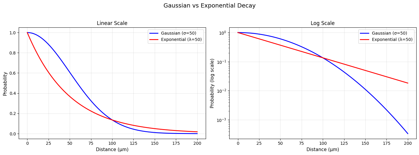
📊 Key differences:
  Gaussian: Symmetric, bell-shaped, faster tail decay
  Exponential: Monotonic, linear in log-space, heavier tails
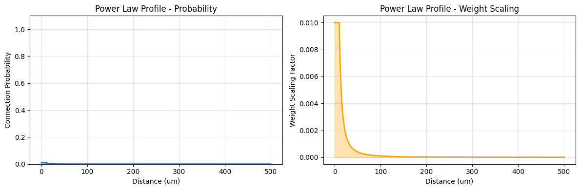
2.3 Power Law Profile#
The Power Law profile follows:
Parameters:
exponent(α): Power law exponentmin_distance: Avoid division by zeromax_distance: Optional cutoff
Use cases:
Scale-free networks
Long-range connections
Brain-wide connectivity
# Create Power Law profile
powerlaw = init.PowerLawProfile(
exponent=2.0,
min_distance=10.0 * u.um,
max_distance=500.0 * u.um
)
visualize_profile(powerlaw, max_distance=500, title="Power Law Profile")
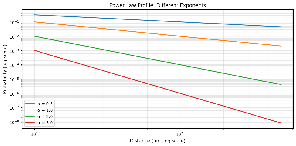
# Compare different exponents
fig, ax = plt.subplots(1, 1, figsize=(10, 5))
distances = np.linspace(10, 500, 500) * u.um
exponents = [0.5, 1.0, 2.0, 3.0]
for exp in exponents:
profile = init.PowerLawProfile(exponent=exp, min_distance=10.0 * u.um)
probs = profile.probability(distances)
ax.loglog(distances.mantissa, probs, linewidth=2, label=f'α = {exp}')
ax.set_xlabel('Distance (μm, log scale)', fontsize=11)
ax.set_ylabel('Probability (log scale)', fontsize=11)
ax.set_title('Power Law Profile: Different Exponents', fontsize=12)
ax.legend()
ax.grid(alpha=0.3, which='both')
plt.tight_layout()
plt.show()
print("\n💡 Power law properties:")
print(" - Linear in log-log space")
print(" - Larger α → steeper decay")
print(" - Heavy tails (scale-free)")
💡 Power law properties:
  - Linear in log-log space
  - Larger α → steeper decay
  - Heavy tails (scale-free)
2.4 Linear Profile#
The Linear profile decreases linearly:
Parameters:
max_distance: Distance at which probability reaches 0
Use cases:
Simple distance decay
Hard cutoffs
Piecewise connectivity
# Create Linear profile
linear = init.LinearProfile(max_distance=150.0 * u.um)

visualize_profile(linear, max_distance=200, title="Linear Profile")

print("\nLinear Profile Properties:")
print("  - Simplest decay pattern")
print("  - Hard cutoff at max_distance")
print("  - Uniform rate of decay")
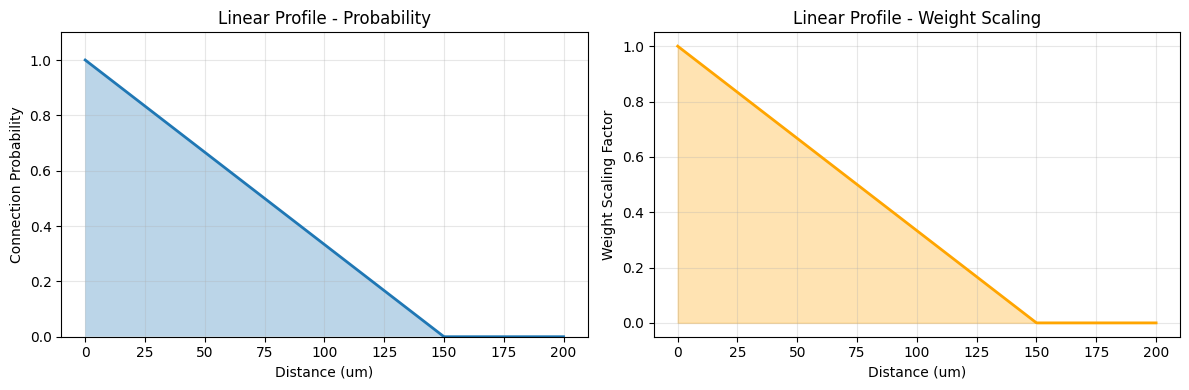
Linear Profile Properties:
  - Simplest decay pattern
  - Hard cutoff at max_distance
  - Uniform rate of decay
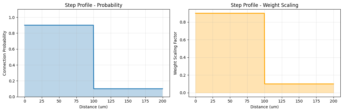
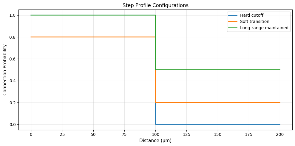
2.5 Step Profile#
The Step profile creates binary connectivity regions:
Parameters:
threshold: Distance thresholdinside_prob: Probability inside thresholdoutside_prob: Probability outside threshold
Use cases:
Local vs long-range separation
Two-population connectivity
Binary spatial domains
# Create Step profile
step = init.StepProfile(
    threshold=100.0 * u.um,
    inside_prob=0.9,
    outside_prob=0.1
)

visualize_profile(step, max_distance=200, title="Step Profile")

# Compare different step configurations
fig, ax = plt.subplots(1, 1, figsize=(10, 5))

distances = np.linspace(0, 200, 1000) * u.um

configs = [
    (100.0, 1.0, 0.0, 'Hard cutoff'),
    (100.0, 0.8, 0.2, 'Soft transition'),
    (100.0, 1.0, 0.5, 'Long-range maintained'),
]

for threshold, p_in, p_out, label in configs:
    profile = init.StepProfile(threshold * u.um, p_in, p_out)
    probs = profile.probability(distances)
    ax.plot(distances.mantissa, probs, linewidth=2, label=label)

ax.set_xlabel('Distance (μm)', fontsize=11)
ax.set_ylabel('Connection Probability', fontsize=11)
ax.set_title('Step Profile Configurations', fontsize=12)
ax.legend()
ax.grid(alpha=0.3)

plt.tight_layout()
plt.show()
3. Advanced Distance Profiles#
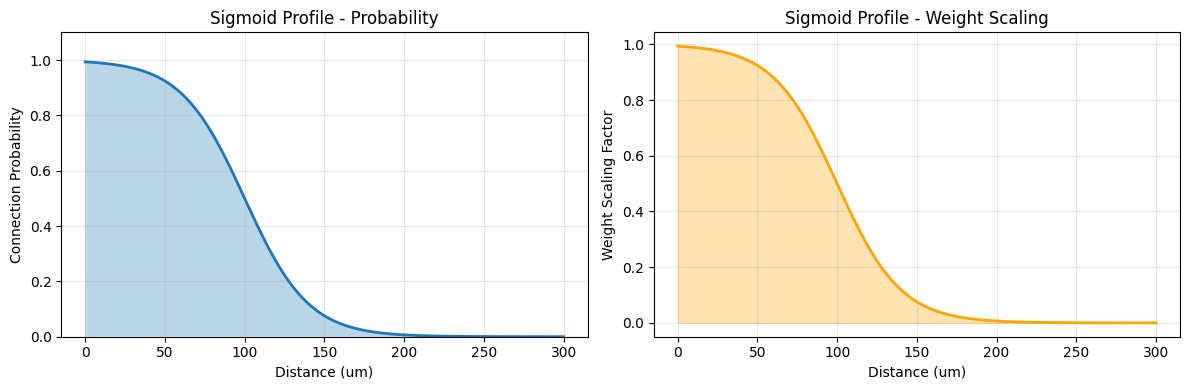
3.1 Sigmoid Profile#
The Sigmoid profile creates smooth S-shaped transitions:
Parameters:
midpoint: Distance at which probability is 0.5slope: Steepness of transitionmax_distance: Optional cutoff
Use cases:
Smooth transitions
Threshold-like behavior
Gradual connectivity changes
# Create Sigmoid profile
sigmoid = init.SigmoidProfile(
    midpoint=100.0 * u.um,
    slope=0.05,
    max_distance=300.0 * u.um
)

visualize_profile(sigmoid, max_distance=300, title="Sigmoid Profile")

# Compare different slopes
fig, ax = plt.subplots(1, 1, figsize=(10, 5))

distances = np.linspace(0, 250, 500) * u.um
slopes = [0.01, 0.05, 0.1, 0.2]

for slope in slopes:
    profile = init.SigmoidProfile(midpoint=100.0 * u.um, slope=slope)
    probs = profile.probability(distances)
    ax.plot(distances.mantissa, probs, linewidth=2, label=f'slope = {slope}')

ax.axvline(100, color='red', linestyle='--', alpha=0.5, label='Midpoint')
ax.axhline(0.5, color='red', linestyle='--', alpha=0.5)
ax.set_xlabel('Distance (μm)', fontsize=11)
ax.set_ylabel('Connection Probability', fontsize=11)
ax.set_title('Sigmoid Profile: Effect of Slope', fontsize=12)
ax.legend()
ax.grid(alpha=0.3)

plt.tight_layout()
plt.show()

print("\n💡 Larger slope → sharper transition (approaches step function)")
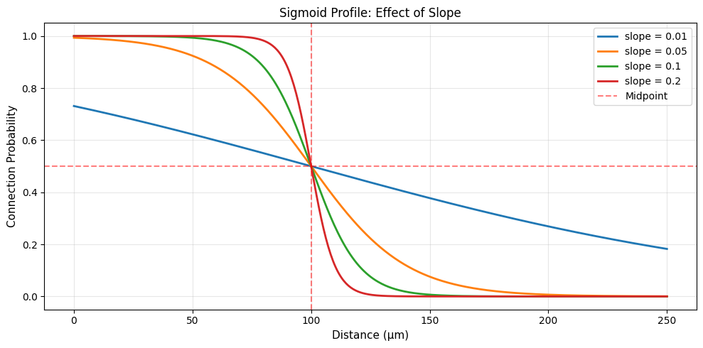
💡 Larger slope → sharper transition (approaches step function)
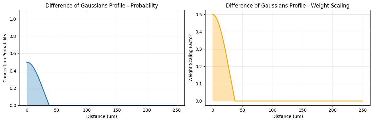
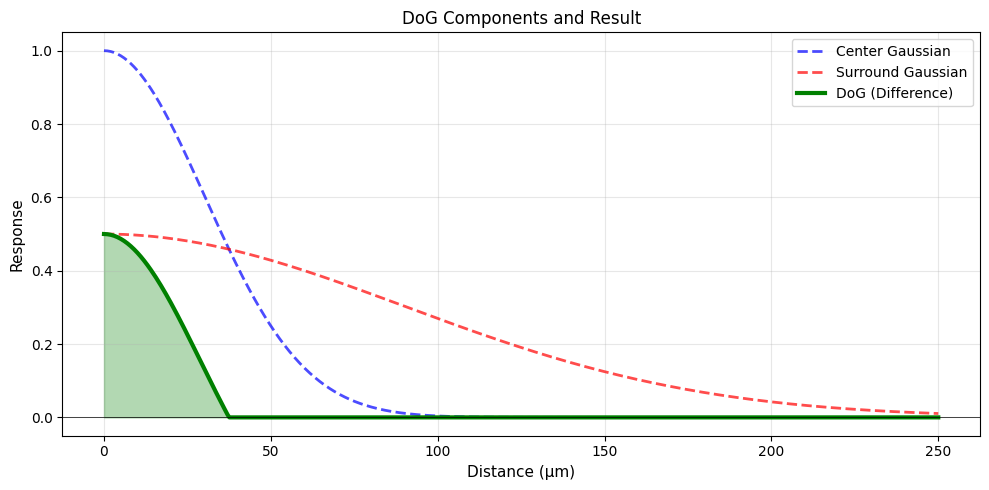
3.2 Difference of Gaussians (DoG) Profile#
The DoG profile creates center-surround patterns:
Parameters:
sigma_center: Center Gaussian widthsigma_surround: Surround Gaussian width (> sigma_center)amplitude_center: Center amplitudeamplitude_surround: Surround amplitude
Use cases:
Lateral inhibition
Center-surround receptive fields
Competitive dynamics
# Create DoG profile
dog = init.DoGProfile(
    sigma_center=30.0 * u.um,
    sigma_surround=90.0 * u.um,
    amplitude_center=1.0,
    amplitude_surround=0.5,
    max_distance=250.0 * u.um
)

visualize_profile(dog, max_distance=250, title="Difference of Gaussians Profile")

# Visualize components
fig, ax = plt.subplots(1, 1, figsize=(10, 5))

distances = np.linspace(0, 250, 500) * u.um

# Components
center_gaussian = init.GaussianProfile(sigma=30.0 * u.um)
surround_gaussian = init.GaussianProfile(sigma=90.0 * u.um)

center = center_gaussian.probability(distances)
surround = 0.5 * surround_gaussian.probability(distances)
dog_result = dog.probability(distances)

ax.plot(distances.mantissa, center, 'b--', linewidth=2, label='Center Gaussian', alpha=0.7)
ax.plot(distances.mantissa, surround, 'r--', linewidth=2, label='Surround Gaussian', alpha=0.7)
ax.plot(distances.mantissa, dog_result, 'g-', linewidth=3, label='DoG (Difference)')
ax.axhline(0, color='black', linestyle='-', linewidth=0.5)
ax.fill_between(distances.mantissa, 0, dog_result, alpha=0.3, color='green')

ax.set_xlabel('Distance (μm)', fontsize=11)
ax.set_ylabel('Response', fontsize=11)
ax.set_title('DoG Components and Result', fontsize=12)
ax.legend()
ax.grid(alpha=0.3)

plt.tight_layout()
plt.show()

print("\n🧠 DoG creates lateral inhibition:")
print("  - Strong excitation at center")
print("  - Inhibition at intermediate distances")
print("  - Common in visual cortex receptive fields")
🧠 DoG creates lateral inhibition:
  - Strong excitation at center
  - Inhibition at intermediate distances
  - Common in visual cortex receptive fields
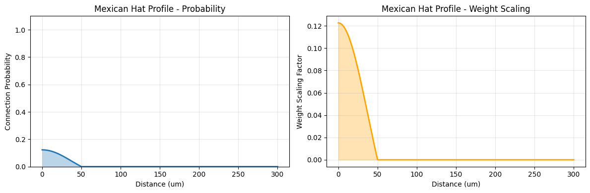
3.3 Mexican Hat Profile#
The Mexican Hat profile is the second derivative of a Gaussian:
Parameters:
sigma: Width parameteramplitude: Scaling factormax_distance: Optional cutoff
Use cases:
Center-surround patterns
Lateral inhibition
Self-organizing maps
# Create Mexican Hat profile
mexican_hat = init.MexicanHatProfile(
sigma=50.0 * u.um,
amplitude=1.0,
max_distance=300.0 * u.um
)
visualize_profile(mexican_hat, max_distance=300, title="Mexican Hat Profile")
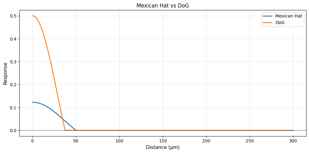
# Compare with DoG
fig, ax = plt.subplots(1, 1, figsize=(10, 5))
distances = np.linspace(0, 300, 500) * u.um
mh_profile = init.MexicanHatProfile(sigma=50.0 * u.um)
dog_profile = init.DoGProfile(sigma_center=30.0 * u.um, sigma_surround=90.0 * u.um)
mh_prob = mh_profile.probability(distances)
dog_prob = dog_profile.probability(distances)
ax.plot(distances.mantissa, mh_prob, linewidth=2, label='Mexican Hat')
ax.plot(distances.mantissa, dog_prob, linewidth=2, label='DoG')
ax.axhline(0, color='black', linestyle='-', linewidth=0.5)
ax.set_xlabel('Distance (μm)', fontsize=11)
ax.set_ylabel('Response', fontsize=11)
ax.set_title('Mexican Hat vs DoG', fontsize=12)
ax.legend()
ax.grid(alpha=0.3)
plt.tight_layout()
plt.show()
print("\n📊 Mexican Hat properties:")
print(" - Single parameter (sigma) controls shape")
print(" - More regular than DoG")
print(" - Ricker wavelet in signal processing")
📊 Mexican Hat properties:
  - Single parameter (sigma) controls shape
  - More regular than DoG
  - Ricker wavelet in signal processing
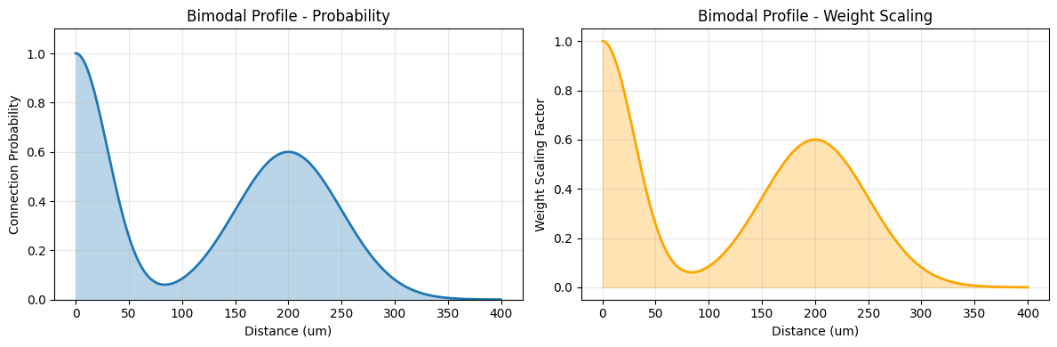
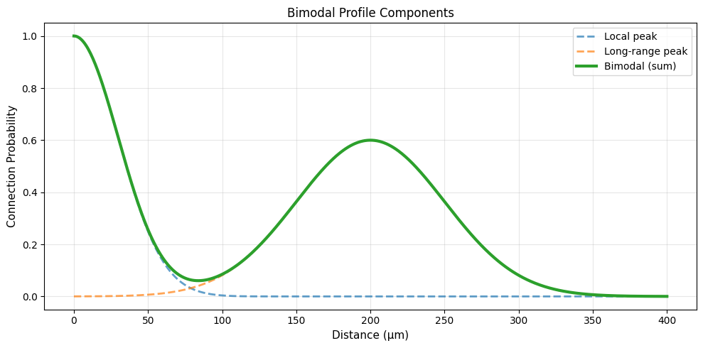
3.4 Bimodal Profile#
The Bimodal profile has two peaks:
Parameters:
sigma1,sigma2: Widths of two peakscenter1,center2: Locations of peaksamplitude1,amplitude2: Heights of peaks
Use cases:
Local + long-range connections
Multi-scale connectivity
Hierarchical networks
# Create Bimodal profile
bimodal = init.BimodalProfile(
    sigma1=30.0 * u.um,
    sigma2=50.0 * u.um,
    center1=0.0 * u.um,
    center2=200.0 * u.um,
    amplitude1=1.0,
    amplitude2=0.6,
    max_distance=400.0 * u.um
)

visualize_profile(bimodal, max_distance=400, title="Bimodal Profile")

# Show components
fig, ax = plt.subplots(1, 1, figsize=(10, 5))

distances = np.linspace(0, 400, 500) * u.um

# Individual Gaussians
gauss1 = init.GaussianProfile(sigma=30.0 * u.um)
gauss2 = init.GaussianProfile(sigma=50.0 * u.um)

prob1 = gauss1.probability(distances)
prob2 = 0.6 * gauss2.probability(distances - 200.0 * u.um + distances[0])
bimodal_prob = bimodal.probability(distances)

ax.plot(distances.mantissa, prob1, '--', linewidth=2, label='Local peak', alpha=0.7)
ax.plot(distances.mantissa, prob2, '--', linewidth=2, label='Long-range peak', alpha=0.7)
ax.plot(distances.mantissa, bimodal_prob, linewidth=3, label='Bimodal (sum)')

ax.set_xlabel('Distance (μm)', fontsize=11)
ax.set_ylabel('Connection Probability', fontsize=11)
ax.set_title('Bimodal Profile Components', fontsize=12)
ax.legend()
ax.grid(alpha=0.3)

plt.tight_layout()
plt.show()

print("\n🔗 Bimodal connectivity:")
print("  - Local connections (first peak)")
print("  - Long-range connections (second peak)")
print("  - Common in cortical circuits")
🔗 Bimodal connectivity:
  - Local connections (first peak)
  - Long-range connections (second peak)
  - Common in cortical circuits
3.5 Logistic Profile#
The Logistic profile is similar to sigmoid:
Parameters:
growth_rate: Controls decay speedmidpoint: Half-probability distance
Use cases:
Growth-like patterns
Smooth transitions
Similar to sigmoid
# Create Logistic profile
logistic = init.LogisticProfile(
    growth_rate=0.05,
    midpoint=100.0 * u.um,
    max_distance=300.0 * u.um
)

visualize_profile(logistic, max_distance=300, title="Logistic Profile")

(ArrayImpl([  0.       ,   0.60120243,   1.20240486,   1.80360723,
              2.40480971,   3.00601... * umetre,
 array([9.93307149e-01, 9.93104315e-01, 9.92895378e-01, 9.92680157e-01,
        9.92458466e-01, 9.92230113e-01, 9.91994901e-01, 9.91752628e-01,
        9.91503086e-01, 9.91246060e-01, 9.90981330e-01, 9.90708669e-01,
        9.90427844e-01, 9.90138616e-01, 9.89840739e-01, 9.89533958e-01,
        9.89218015e-01, 9.88892641e-01, 9.88557562e-01, 9.88212495e-01,
        9.87857150e-01, 9.87491228e-01, 9.87114423e-01, 9.86726420e-01,
        9.86326896e-01, 9.85915517e-01, 9.85491944e-01, 9.85055825e-01,
        9.84606802e-01, 9.84144503e-01, 9.83668551e-01, 9.83178556e-01,
        9.82674119e-01, 9.82154829e-01, 9.81620266e-01, 9.81069999e-01,
        9.80503584e-01, 9.79920569e-01, 9.79320487e-01, 9.78702860e-01,
        9.78067201e-01, 9.77413007e-01, 9.76739764e-01, 9.76046945e-01,
        9.75334012e-01, 9.74600412e-01, 9.73845578e-01, 9.73068932e-01,
        9.72269880e-01, 9.71447816e-01, 9.70602118e-01, 9.69732152e-01,
        9.68837267e-01, 9.67916801e-01, 9.66970073e-01, 9.65996390e-01,
        9.64995042e-01, 9.63965307e-01, 9.62906445e-01, 9.61817701e-01,
        9.60698305e-01, 9.59547473e-01, 9.58364401e-01, 9.57148275e-01,
        9.55898262e-01, 9.54613515e-01, 9.53293169e-01, 9.51936347e-01,
        9.50542155e-01, 9.49109683e-01, 9.47638007e-01, 9.46126188e-01,
        9.44573273e-01, 9.42978292e-01, 9.41340264e-01, 9.39658192e-01,
        9.37931067e-01, 9.36157866e-01, 9.34337554e-01, 9.32469085e-01,
        9.30551399e-01, 9.28583426e-01, 9.26564088e-01, 9.24492296e-01,
        9.22366950e-01, 9.20186946e-01, 9.17951171e-01, 9.15658507e-01,
        9.13307830e-01, 9.10898012e-01, 9.08427925e-01, 9.05896435e-01,
        9.03302412e-01, 9.00644726e-01, 8.97922249e-01, 8.95133859e-01,
        8.92278437e-01, 8.89354875e-01, 8.86362073e-01, 8.83298943e-01,
        8.80164408e-01, 8.76957408e-01, 8.73676902e-01, 8.70321866e-01,
        8.66891299e-01, 8.63384223e-01, 8.59799690e-01, 8.56136776e-01,
        8.52394593e-01, 8.48572285e-01, 8.44669034e-01, 8.40684061e-01,
        8.36616630e-01, 8.32466049e-01, 8.28231675e-01, 8.23912916e-01,
        8.19509235e-01, 8.15020149e-01, 8.10445238e-01, 8.05784143e-01,
        8.01036571e-01, 7.96202298e-01, 7.91281170e-01, 7.86273109e-01,
        7.81178114e-01, 7.75996263e-01, 7.70727717e-01, 7.65372722e-01,
        7.59931611e-01, 7.54404809e-01, 7.48792829e-01, 7.43096283e-01,
        7.37315874e-01, 7.31452408e-01, 7.25506786e-01, 7.19480013e-01,
        7.13373192e-01, 7.07187534e-01, 7.00924349e-01, 6.94585053e-01,
        6.88171166e-01, 6.81684312e-01, 6.75126219e-01, 6.68498719e-01,
        6.61803744e-01, 6.55043329e-01, 6.48219608e-01, 6.41334813e-01,
        6.34391273e-01, 6.27391408e-01, 6.20337731e-01, 6.13232840e-01,
        6.06079421e-01, 5.98880239e-01, 5.91638135e-01, 5.84356025e-01,
        5.77036892e-01, 5.69683785e-01, 5.62299811e-01, 5.54888130e-01,
        5.47451953e-01, 5.39994533e-01, 5.32519162e-01, 5.25029162e-01,
        5.17527885e-01, 5.10018699e-01, 5.02504989e-01, 4.94990148e-01,
        4.87477569e-01, 4.79970644e-01, 4.72472752e-01, 4.64987258e-01,
        4.57517503e-01, 4.50066800e-01, 4.42638429e-01, 4.35235629e-01,
        4.27861595e-01, 4.20519470e-01, 4.13212343e-01, 4.05943240e-01,
        3.98715123e-01, 3.91530883e-01, 3.84393337e-01, 3.77305223e-01,
        3.70269199e-01, 3.63287834e-01, 3.56363611e-01, 3.49498920e-01,
        3.42696058e-01, 3.35957224e-01, 3.29284520e-01, 3.22679945e-01,
        3.16145400e-01, 3.09682682e-01, 3.03293483e-01, 2.96979394e-01,
        2.90741899e-01, 2.84582379e-01, 2.78502112e-01, 2.72502271e-01,
        2.66583928e-01, 2.60748052e-01, 2.54995514e-01, 2.49327082e-01,
        2.43743432e-01, 2.38245141e-01, 2.32832693e-01, 2.27506482e-01,
        2.22266811e-01, 2.17113898e-01, 2.12047876e-01, 2.07068797e-01,
        2.02176633e-01, 1.97371281e-01, 1.92652563e-01, 1.88020232e-01,
        1.83473972e-01, 1.79013405e-01, 1.74638087e-01, 1.70347519e-01,
        1.66141145e-01, 1.62018354e-01, 1.57978488e-01, 1.54020839e-01,
        1.50144658e-01, 1.46349151e-01, 1.42633488e-01, 1.38996802e-01,
        1.35438191e-01, 1.31956726e-01, 1.28551445e-01, 1.25221365e-01,
        1.21965476e-01, 1.18782748e-01, 1.15672133e-01, 1.12632565e-01,
        1.09662965e-01, 1.06762239e-01, 1.03929285e-01, 1.01162990e-01,
        9.84622352e-02, 9.58258956e-02, 9.32528429e-02, 9.07419463e-02,
        8.82920742e-02, 8.59020955e-02, 8.35708810e-02, 8.12973046e-02,
        7.90802441e-02, 7.69185831e-02, 7.48112110e-02, 7.27570247e-02,
        7.07549292e-02, 6.88038384e-02, 6.69026761e-02, 6.50503762e-02,
        6.32458840e-02, 6.14881562e-02, 5.97761619e-02, 5.81088827e-02,
        5.64853136e-02, 5.49044629e-02, 5.33653530e-02, 5.18670204e-02,
        5.04085161e-02, 4.89889060e-02, 4.76072708e-02, 4.62627062e-02,
        4.49543236e-02, 4.36812494e-02, 4.24426255e-02, 4.12376095e-02,
        4.00653743e-02, 3.89251087e-02, 3.78160168e-02, 3.67373182e-02,
        3.56882481e-02, 3.46680571e-02, 3.36760110e-02, 3.27113909e-02,
        3.17734930e-02, 3.08616284e-02, 2.99751232e-02, 2.91133180e-02,
        2.82755680e-02, 2.74612428e-02, 2.66697263e-02, 2.59004160e-02,
        2.51527237e-02, 2.44260745e-02, 2.37199071e-02, 2.30336732e-02,
        2.23668376e-02, 2.17188782e-02, 2.10892849e-02, 2.04775605e-02,
        1.98832195e-02, 1.93057888e-02, 1.87448066e-02, 1.81998227e-02,
        1.76703982e-02, 1.71561054e-02, 1.66565271e-02, 1.61712570e-02,
        1.56998990e-02, 1.52420672e-02, 1.47973857e-02, 1.43654884e-02,
        1.39460187e-02, 1.35386291e-02, 1.31429815e-02, 1.27587466e-02,
        1.23856039e-02, 1.20232411e-02, 1.16713547e-02, 1.13296489e-02,
        1.09978360e-02, 1.06756360e-02, 1.03627765e-02, 1.00589924e-02,
        9.76402581e-03, 9.47762595e-03, 9.19954877e-03, 8.92955692e-03,
        8.66741959e-03, 8.41291227e-03, 8.16581666e-03, 7.92592049e-03,
        7.69301734e-03, 7.46690655e-03, 7.24739299e-03, 7.03428700e-03,
        6.82740419e-03, 6.62656533e-03, 6.43159620e-03, 6.24232748e-03,
        6.05859458e-03, 5.88023757e-03, 5.70710100e-03, 5.53903383e-03,
        5.37588927e-03, 5.21752470e-03, 5.06380152e-03, 4.91458510e-03,
        4.76974460e-03, 4.62915291e-03, 4.49268656e-03, 4.36022559e-03,
        4.23165345e-03, 4.10685694e-03, 3.98572610e-03, 3.86815411e-03,
        3.75403722e-03, 3.64327465e-03, 3.53576852e-03, 3.43142377e-03,
        3.33014807e-03, 3.23185174e-03, 3.13644771e-03, 3.04385139e-03,
        2.95398067e-03, 2.86675578e-03, 2.78209927e-03, 2.69993593e-03,
        2.62019274e-03, 2.54279877e-03, 2.46768518e-03, 2.39478509e-03,
        2.32403359e-03, 2.25536765e-03, 2.18872606e-03, 2.12404940e-03,
        2.06127999e-03, 2.00036180e-03, 1.94124046e-03, 1.88386318e-03,
        1.82817868e-03, 1.77413723e-03, 1.72169049e-03, 1.67079159e-03,
        1.62139498e-03, 1.57345647e-03, 1.52693315e-03, 1.48178337e-03,
        1.43796670e-03, 1.39544389e-03, 1.35417684e-03, 1.31412856e-03,
        1.27526315e-03, 1.23754576e-03, 1.20094257e-03, 1.16542073e-03,
        1.13094838e-03, 1.09749458e-03, 1.06502930e-03, 1.03352338e-03,
        1.00294855e-03, 9.73277334e-04, 9.44483080e-04, 9.16539919e-04,
        8.89422738e-04, 8.63107166e-04, 8.37569546e-04, 8.12786920e-04,
        7.88737001e-04, 7.65398160e-04, 7.42749406e-04, 7.20770364e-04,
        6.99441258e-04, 6.78742897e-04, 6.58656652e-04, 6.39164446e-04,
        6.20248732e-04, 6.01892480e-04, 5.84079164e-04, 5.66792743e-04,
        5.50017650e-04, 5.33738776e-04, 5.17941459e-04, 5.02611467e-04,
        4.87734989e-04, 4.73298622e-04, 4.59289358e-04, 4.45694572e-04,
        4.32502013e-04, 4.19699789e-04, 4.07276362e-04, 3.95220531e-04,
        3.83521430e-04, 3.72168511e-04, 3.61151536e-04, 3.50460573e-04,
        3.40085981e-04, 3.30018403e-04, 3.20248762e-04, 3.10768244e-04,
        3.01568298e-04, 2.92640628e-04, 2.83977178e-04, 2.75570134e-04,
        2.67411910e-04, 2.59495148e-04, 2.51812703e-04, 2.44357643e-04,
        2.37123243e-04, 2.30102974e-04, 2.23290500e-04, 2.16679674e-04,
        2.10264530e-04, 2.04039277e-04, 1.97998297e-04, 1.92136138e-04,
        1.86447509e-04, 1.80927273e-04, 1.75570449e-04, 1.70372201e-04,
        1.65327836e-04, 1.60432800e-04, 1.55682674e-04, 1.51073169e-04,
        1.46600124e-04, 1.42259500e-04, 1.38047379e-04, 1.33959956e-04,
        1.29993541e-04, 1.26144553e-04, 1.22409516e-04, 1.18785057e-04,
        1.15267903e-04, 1.11854879e-04, 1.08542901e-04, 1.05328979e-04,
        1.02210211e-04, 9.91837803e-05, 9.62469527e-05, 9.33970764e-05,
        9.06315773e-05, 8.79479578e-05, 8.53437941e-05, 8.28167340e-05,
        8.03644951e-05, 7.79848623e-05, 7.56756863e-05, 7.34348813e-05,
        7.12604232e-05, 6.91503479e-05, 6.71027493e-05, 6.51157778e-05,
        6.31876386e-05, 6.13165900e-05, 5.95009416e-05, 5.77390534e-05,
        5.60293336e-05, 5.43702380e-05, 5.27602675e-05, 5.11979678e-05,
        4.96819275e-05, 4.82107771e-05, 4.67831874e-05, 4.53978687e-05]),
 array([9.93307149e-01, 9.93104315e-01, 9.92895378e-01, 9.92680157e-01,
        9.92458466e-01, 9.92230113e-01, 9.91994901e-01, 9.91752628e-01,
        9.91503086e-01, 9.91246060e-01, 9.90981330e-01, 9.90708669e-01,
        9.90427844e-01, 9.90138616e-01, 9.89840739e-01, 9.89533958e-01,
        9.89218015e-01, 9.88892641e-01, 9.88557562e-01, 9.88212495e-01,
        9.87857150e-01, 9.87491228e-01, 9.87114423e-01, 9.86726420e-01,
        9.86326896e-01, 9.85915517e-01, 9.85491944e-01, 9.85055825e-01,
        9.84606802e-01, 9.84144503e-01, 9.83668551e-01, 9.83178556e-01,
        9.82674119e-01, 9.82154829e-01, 9.81620266e-01, 9.81069999e-01,
        9.80503584e-01, 9.79920569e-01, 9.79320487e-01, 9.78702860e-01,
        9.78067201e-01, 9.77413007e-01, 9.76739764e-01, 9.76046945e-01,
        9.75334012e-01, 9.74600412e-01, 9.73845578e-01, 9.73068932e-01,
        9.72269880e-01, 9.71447816e-01, 9.70602118e-01, 9.69732152e-01,
        9.68837267e-01, 9.67916801e-01, 9.66970073e-01, 9.65996390e-01,
        9.64995042e-01, 9.63965307e-01, 9.62906445e-01, 9.61817701e-01,
        9.60698305e-01, 9.59547473e-01, 9.58364401e-01, 9.57148275e-01,
        9.55898262e-01, 9.54613515e-01, 9.53293169e-01, 9.51936347e-01,
        9.50542155e-01, 9.49109683e-01, 9.47638007e-01, 9.46126188e-01,
        9.44573273e-01, 9.42978292e-01, 9.41340264e-01, 9.39658192e-01,
        9.37931067e-01, 9.36157866e-01, 9.34337554e-01, 9.32469085e-01,
        9.30551399e-01, 9.28583426e-01, 9.26564088e-01, 9.24492296e-01,
        9.22366950e-01, 9.20186946e-01, 9.17951171e-01, 9.15658507e-01,
        9.13307830e-01, 9.10898012e-01, 9.08427925e-01, 9.05896435e-01,
        9.03302412e-01, 9.00644726e-01, 8.97922249e-01, 8.95133859e-01,
        8.92278437e-01, 8.89354875e-01, 8.86362073e-01, 8.83298943e-01,
        8.80164408e-01, 8.76957408e-01, 8.73676902e-01, 8.70321866e-01,
        8.66891299e-01, 8.63384223e-01, 8.59799690e-01, 8.56136776e-01,
        8.52394593e-01, 8.48572285e-01, 8.44669034e-01, 8.40684061e-01,
        8.36616630e-01, 8.32466049e-01, 8.28231675e-01, 8.23912916e-01,
        8.19509235e-01, 8.15020149e-01, 8.10445238e-01, 8.05784143e-01,
        8.01036571e-01, 7.96202298e-01, 7.91281170e-01, 7.86273109e-01,
        7.81178114e-01, 7.75996263e-01, 7.70727717e-01, 7.65372722e-01,
        7.59931611e-01, 7.54404809e-01, 7.48792829e-01, 7.43096283e-01,
        7.37315874e-01, 7.31452408e-01, 7.25506786e-01, 7.19480013e-01,
        7.13373192e-01, 7.07187534e-01, 7.00924349e-01, 6.94585053e-01,
        6.88171166e-01, 6.81684312e-01, 6.75126219e-01, 6.68498719e-01,
        6.61803744e-01, 6.55043329e-01, 6.48219608e-01, 6.41334813e-01,
        6.34391273e-01, 6.27391408e-01, 6.20337731e-01, 6.13232840e-01,
        6.06079421e-01, 5.98880239e-01, 5.91638135e-01, 5.84356025e-01,
        5.77036892e-01, 5.69683785e-01, 5.62299811e-01, 5.54888130e-01,
        5.47451953e-01, 5.39994533e-01, 5.32519162e-01, 5.25029162e-01,
        5.17527885e-01, 5.10018699e-01, 5.02504989e-01, 4.94990148e-01,
        4.87477569e-01, 4.79970644e-01, 4.72472752e-01, 4.64987258e-01,
        4.57517503e-01, 4.50066800e-01, 4.42638429e-01, 4.35235629e-01,
        4.27861595e-01, 4.20519470e-01, 4.13212343e-01, 4.05943240e-01,
        3.98715123e-01, 3.91530883e-01, 3.84393337e-01, 3.77305223e-01,
        3.70269199e-01, 3.63287834e-01, 3.56363611e-01, 3.49498920e-01,
        3.42696058e-01, 3.35957224e-01, 3.29284520e-01, 3.22679945e-01,
        3.16145400e-01, 3.09682682e-01, 3.03293483e-01, 2.96979394e-01,
        2.90741899e-01, 2.84582379e-01, 2.78502112e-01, 2.72502271e-01,
        2.66583928e-01, 2.60748052e-01, 2.54995514e-01, 2.49327082e-01,
        2.43743432e-01, 2.38245141e-01, 2.32832693e-01, 2.27506482e-01,
        2.22266811e-01, 2.17113898e-01, 2.12047876e-01, 2.07068797e-01,
        2.02176633e-01, 1.97371281e-01, 1.92652563e-01, 1.88020232e-01,
        1.83473972e-01, 1.79013405e-01, 1.74638087e-01, 1.70347519e-01,
        1.66141145e-01, 1.62018354e-01, 1.57978488e-01, 1.54020839e-01,
        1.50144658e-01, 1.46349151e-01, 1.42633488e-01, 1.38996802e-01,
        1.35438191e-01, 1.31956726e-01, 1.28551445e-01, 1.25221365e-01,
        1.21965476e-01, 1.18782748e-01, 1.15672133e-01, 1.12632565e-01,
        1.09662965e-01, 1.06762239e-01, 1.03929285e-01, 1.01162990e-01,
        9.84622352e-02, 9.58258956e-02, 9.32528429e-02, 9.07419463e-02,
        8.82920742e-02, 8.59020955e-02, 8.35708810e-02, 8.12973046e-02,
        7.90802441e-02, 7.69185831e-02, 7.48112110e-02, 7.27570247e-02,
        7.07549292e-02, 6.88038384e-02, 6.69026761e-02, 6.50503762e-02,
        6.32458840e-02, 6.14881562e-02, 5.97761619e-02, 5.81088827e-02,
        5.64853136e-02, 5.49044629e-02, 5.33653530e-02, 5.18670204e-02,
        5.04085161e-02, 4.89889060e-02, 4.76072708e-02, 4.62627062e-02,
        4.49543236e-02, 4.36812494e-02, 4.24426255e-02, 4.12376095e-02,
        4.00653743e-02, 3.89251087e-02, 3.78160168e-02, 3.67373182e-02,
        3.56882481e-02, 3.46680571e-02, 3.36760110e-02, 3.27113909e-02,
        3.17734930e-02, 3.08616284e-02, 2.99751232e-02, 2.91133180e-02,
        2.82755680e-02, 2.74612428e-02, 2.66697263e-02, 2.59004160e-02,
        2.51527237e-02, 2.44260745e-02, 2.37199071e-02, 2.30336732e-02,
        2.23668376e-02, 2.17188782e-02, 2.10892849e-02, 2.04775605e-02,
        1.98832195e-02, 1.93057888e-02, 1.87448066e-02, 1.81998227e-02,
        1.76703982e-02, 1.71561054e-02, 1.66565271e-02, 1.61712570e-02,
        1.56998990e-02, 1.52420672e-02, 1.47973857e-02, 1.43654884e-02,
        1.39460187e-02, 1.35386291e-02, 1.31429815e-02, 1.27587466e-02,
        1.23856039e-02, 1.20232411e-02, 1.16713547e-02, 1.13296489e-02,
        1.09978360e-02, 1.06756360e-02, 1.03627765e-02, 1.00589924e-02,
        9.76402581e-03, 9.47762595e-03, 9.19954877e-03, 8.92955692e-03,
        8.66741959e-03, 8.41291227e-03, 8.16581666e-03, 7.92592049e-03,
        7.69301734e-03, 7.46690655e-03, 7.24739299e-03, 7.03428700e-03,
        6.82740419e-03, 6.62656533e-03, 6.43159620e-03, 6.24232748e-03,
        6.05859458e-03, 5.88023757e-03, 5.70710100e-03, 5.53903383e-03,
        5.37588927e-03, 5.21752470e-03, 5.06380152e-03, 4.91458510e-03,
        4.76974460e-03, 4.62915291e-03, 4.49268656e-03, 4.36022559e-03,
        4.23165345e-03, 4.10685694e-03, 3.98572610e-03, 3.86815411e-03,
        3.75403722e-03, 3.64327465e-03, 3.53576852e-03, 3.43142377e-03,
        3.33014807e-03, 3.23185174e-03, 3.13644771e-03, 3.04385139e-03,
        2.95398067e-03, 2.86675578e-03, 2.78209927e-03, 2.69993593e-03,
        2.62019274e-03, 2.54279877e-03, 2.46768518e-03, 2.39478509e-03,
        2.32403359e-03, 2.25536765e-03, 2.18872606e-03, 2.12404940e-03,
        2.06127999e-03, 2.00036180e-03, 1.94124046e-03, 1.88386318e-03,
        1.82817868e-03, 1.77413723e-03, 1.72169049e-03, 1.67079159e-03,
        1.62139498e-03, 1.57345647e-03, 1.52693315e-03, 1.48178337e-03,
        1.43796670e-03, 1.39544389e-03, 1.35417684e-03, 1.31412856e-03,
        1.27526315e-03, 1.23754576e-03, 1.20094257e-03, 1.16542073e-03,
        1.13094838e-03, 1.09749458e-03, 1.06502930e-03, 1.03352338e-03,
        1.00294855e-03, 9.73277334e-04, 9.44483080e-04, 9.16539919e-04,
        8.89422738e-04, 8.63107166e-04, 8.37569546e-04, 8.12786920e-04,
        7.88737001e-04, 7.65398160e-04, 7.42749406e-04, 7.20770364e-04,
        6.99441258e-04, 6.78742897e-04, 6.58656652e-04, 6.39164446e-04,
        6.20248732e-04, 6.01892480e-04, 5.84079164e-04, 5.66792743e-04,
        5.50017650e-04, 5.33738776e-04, 5.17941459e-04, 5.02611467e-04,
        4.87734989e-04, 4.73298622e-04, 4.59289358e-04, 4.45694572e-04,
        4.32502013e-04, 4.19699789e-04, 4.07276362e-04, 3.95220531e-04,
        3.83521430e-04, 3.72168511e-04, 3.61151536e-04, 3.50460573e-04,
        3.40085981e-04, 3.30018403e-04, 3.20248762e-04, 3.10768244e-04,
        3.01568298e-04, 2.92640628e-04, 2.83977178e-04, 2.75570134e-04,
        2.67411910e-04, 2.59495148e-04, 2.51812703e-04, 2.44357643e-04,
        2.37123243e-04, 2.30102974e-04, 2.23290500e-04, 2.16679674e-04,
        2.10264530e-04, 2.04039277e-04, 1.97998297e-04, 1.92136138e-04,
        1.86447509e-04, 1.80927273e-04, 1.75570449e-04, 1.70372201e-04,
        1.65327836e-04, 1.60432800e-04, 1.55682674e-04, 1.51073169e-04,
        1.46600124e-04, 1.42259500e-04, 1.38047379e-04, 1.33959956e-04,
        1.29993541e-04, 1.26144553e-04, 1.22409516e-04, 1.18785057e-04,
        1.15267903e-04, 1.11854879e-04, 1.08542901e-04, 1.05328979e-04,
        1.02210211e-04, 9.91837803e-05, 9.62469527e-05, 9.33970764e-05,
        9.06315773e-05, 8.79479578e-05, 8.53437941e-05, 8.28167340e-05,
        8.03644951e-05, 7.79848623e-05, 7.56756863e-05, 7.34348813e-05,
        7.12604232e-05, 6.91503479e-05, 6.71027493e-05, 6.51157778e-05,
        6.31876386e-05, 6.13165900e-05, 5.95009416e-05, 5.77390534e-05,
        5.60293336e-05, 5.43702380e-05, 5.27602675e-05, 5.11979678e-05,
        4.96819275e-05, 4.82107771e-05, 4.67831874e-05, 4.53978687e-05]))
4. Profile Composition#
One of the most powerful features of distance profiles is the ability to compose them using arithmetic operations and transformations.
4.1 Arithmetic Operations#
Profiles support standard arithmetic operations:
Addition (
+): Combine connectivity patternsSubtraction (
-): Create inhibitory patternsMultiplication (
*): Scale or modulateDivision (
/): Normalize or ratio
# Create base profiles
local = init.GaussianProfile(sigma=30.0 * u.um)
distant = init.GaussianProfile(sigma=100.0 * u.um)

# Compose profiles
combined_add = local + distant * 0.3
combined_sub = local - distant * 0.2
scaled = local * 0.5

# Visualize
fig, axes = plt.subplots(2, 2, figsize=(14, 10))
axes = axes.flatten()

distances = np.linspace(0, 250, 500) * u.um

# Addition
prob_local = local.probability(distances)
prob_distant = distant.probability(distances)
prob_add = combined_add.probability(distances)

axes[0].plot(distances.mantissa, prob_local, '--', label='Local', alpha=0.7)
axes[0].plot(distances.mantissa, prob_distant * 0.3, '--', label='Distant × 0.3', alpha=0.7)
axes[0].plot(distances.mantissa, prob_add, linewidth=2, label='Sum')
axes[0].set_title('Addition: Local + Distant')
axes[0].set_xlabel('Distance (μm)')
axes[0].set_ylabel('Probability')
axes[0].legend()
axes[0].grid(alpha=0.3)

# Subtraction
prob_sub = combined_sub.probability(distances)
axes[1].plot(distances.mantissa, prob_local, '--', label='Local', alpha=0.7)
axes[1].plot(distances.mantissa, prob_distant * 0.2, '--', label='Distant × 0.2', alpha=0.7)
axes[1].plot(distances.mantissa, prob_sub, linewidth=2, label='Difference')
axes[1].axhline(0, color='black', linestyle='-', linewidth=0.5)
axes[1].set_title('Subtraction: Local - Distant')
axes[1].set_xlabel('Distance (μm)')
axes[1].set_ylabel('Probability')
axes[1].legend()
axes[1].grid(alpha=0.3)

# Scaling
prob_scaled = scaled.probability(distances)
axes[2].plot(distances.mantissa, prob_local, '--', label='Original', alpha=0.7)
axes[2].plot(distances.mantissa, prob_scaled, linewidth=2, label='Scaled × 0.5')
axes[2].set_title('Scaling: Profile × 0.5')
axes[2].set_xlabel('Distance (μm)')
axes[2].set_ylabel('Probability')
axes[2].legend()
axes[2].grid(alpha=0.3)

# Complex composition
complex_profile = (local * 0.8) + (distant * 0.3) - (init.GaussianProfile(sigma=60.0 * u.um) * 0.1)
prob_complex = complex_profile.probability(distances)
axes[3].plot(distances.mantissa, prob_complex, linewidth=2, color='purple')
axes[3].fill_between(distances.mantissa, prob_complex, alpha=0.3, color='purple')
axes[3].set_title('Complex: 0.8×Local + 0.3×Distant - 0.1×Medium')
axes[3].set_xlabel('Distance (μm)')
axes[3].set_ylabel('Probability')
axes[3].grid(alpha=0.3)

plt.suptitle('Profile Composition with Arithmetic Operations', fontsize=14, y=1.00)
plt.tight_layout()
plt.show()

print("\n✨ Arithmetic operations enable complex connectivity patterns!")
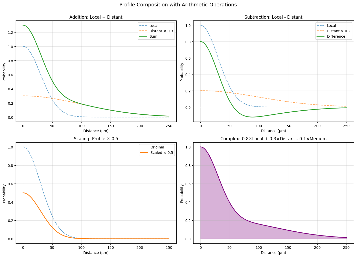
✨ Arithmetic operations enable complex connectivity patterns!
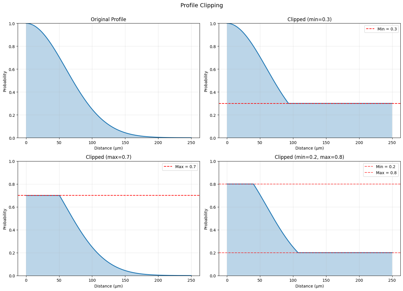
4.2 Clipping Transformations#
The .clip() method bounds profile values:
clipped = profile.clip(min_val=0.1, max_val=0.9)
# Create profile and apply clipping
original = init.GaussianProfile(sigma=60.0 * u.um)
clipped_min = original.clip(min_val=0.3, max_val=None)
clipped_max = original.clip(min_val=None, max_val=0.7)
clipped_both = original.clip(min_val=0.2, max_val=0.8)

# Visualize
fig, axes = plt.subplots(2, 2, figsize=(14, 10))
axes = axes.flatten()

distances = np.linspace(0, 250, 500) * u.um

# Original
prob_original = original.probability(distances)
axes[0].plot(distances.mantissa, prob_original, linewidth=2)
axes[0].fill_between(distances.mantissa, prob_original, alpha=0.3)
axes[0].set_title('Original Profile')
axes[0].set_xlabel('Distance (μm)')
axes[0].set_ylabel('Probability')
axes[0].grid(alpha=0.3)
axes[0].set_ylim([0, 1])

# Clipped min
prob_min = clipped_min.probability(distances)
axes[1].plot(distances.mantissa, prob_min, linewidth=2)
axes[1].fill_between(distances.mantissa, prob_min, alpha=0.3)
axes[1].axhline(0.3, color='red', linestyle='--', label='Min = 0.3')
axes[1].set_title('Clipped (min=0.3)')
axes[1].set_xlabel('Distance (μm)')
axes[1].set_ylabel('Probability')
axes[1].legend()
axes[1].grid(alpha=0.3)
axes[1].set_ylim([0, 1])

# Clipped max
prob_max = clipped_max.probability(distances)
axes[2].plot(distances.mantissa, prob_max, linewidth=2)
axes[2].fill_between(distances.mantissa, prob_max, alpha=0.3)
axes[2].axhline(0.7, color='red', linestyle='--', label='Max = 0.7')
axes[2].set_title('Clipped (max=0.7)')
axes[2].set_xlabel('Distance (μm)')
axes[2].set_ylabel('Probability')
axes[2].legend()
axes[2].grid(alpha=0.3)
axes[2].set_ylim([0, 1])

# Clipped both
prob_both = clipped_both.probability(distances)
axes[3].plot(distances.mantissa, prob_both, linewidth=2)
axes[3].fill_between(distances.mantissa, prob_both, alpha=0.3)
axes[3].axhline(0.2, color='red', linestyle='--', alpha=0.7, label='Min = 0.2')
axes[3].axhline(0.8, color='red', linestyle='--', alpha=0.7, label='Max = 0.8')
axes[3].set_title('Clipped (min=0.2, max=0.8)')
axes[3].set_xlabel('Distance (μm)')
axes[3].set_ylabel('Probability')
axes[3].legend()
axes[3].grid(alpha=0.3)
axes[3].set_ylim([0, 1])

plt.suptitle('Profile Clipping', fontsize=14, y=1.00)
plt.tight_layout()
plt.show()

print("\n✂️ Clipping use cases:")
print("  - Ensure minimum connectivity")
print("  - Cap maximum connection strength")
print("  - Create plateaus in connectivity")
✂️ Clipping use cases:
  - Ensure minimum connectivity
  - Cap maximum connection strength
  - Create plateaus in connectivity
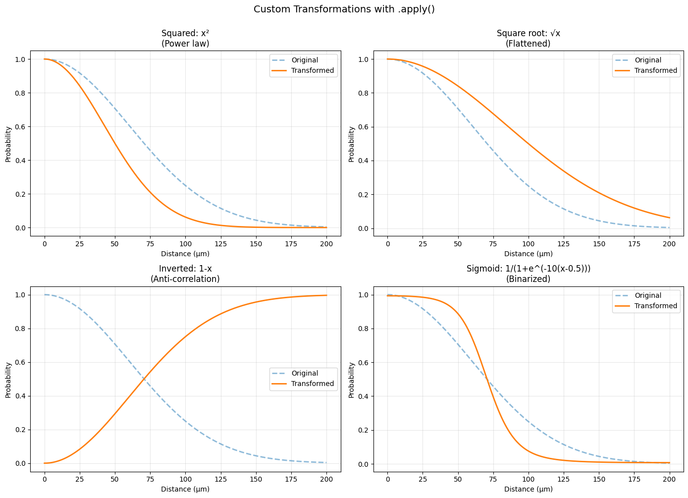
4.3 Apply Transformations#
The .apply() method applies arbitrary functions:
transformed = profile.apply(lambda x: x ** 2)
# Create profile and apply transformations
base = init.GaussianProfile(sigma=60.0 * u.um)

# Different transformations
squared = base.apply(lambda x: x ** 2)
sqrt = base.apply(lambda x: np.sqrt(x))
inverted = base.apply(lambda x: 1 - x)
sigmoid_transform = base.apply(lambda x: 1 / (1 + np.exp(-10 * (x - 0.5))))

# Visualize
fig, axes = plt.subplots(2, 2, figsize=(14, 10))
axes = axes.flatten()

distances = np.linspace(0, 200, 500) * u.um

profiles = [
    (squared, 'Squared: x²', 'Power law'),
    (sqrt, 'Square root: √x', 'Flattened'),
    (inverted, 'Inverted: 1-x', 'Anti-correlation'),
    (sigmoid_transform, 'Sigmoid: 1/(1+e^(-10(x-0.5)))', 'Binarized'),
]

for ax, (profile, title, desc) in zip(axes, profiles):
    prob_original = base.probability(distances)
    prob_transformed = profile.probability(distances)

    ax.plot(distances.mantissa, prob_original, '--', linewidth=2,
            label='Original', alpha=0.5)
    ax.plot(distances.mantissa, prob_transformed, linewidth=2, label='Transformed')
    ax.set_title(f'{title}\n({desc})')
    ax.set_xlabel('Distance (μm)')
    ax.set_ylabel('Probability')
    ax.legend()
    ax.grid(alpha=0.3)

plt.suptitle('Custom Transformations with .apply()', fontsize=14, y=1.00)
plt.tight_layout()
plt.show()

print("\n🔧 Transformation examples:")
print("  x² → Emphasize strong connections")
print("  √x → Flatten differences")
print("  1-x → Create inhibitory pattern")
print("  sigmoid → Binarize connectivity")
🔧 Transformation examples:
  x² → Emphasize strong connections
  √x → Flatten differences
  1-x → Create inhibitory pattern
  sigmoid → Binarize connectivity
4.4 Pipe Operator#
The pipe operator (|) chains operations:
result = profile | (lambda x: x * 2) | (lambda x: np.minimum(x, 1.0))
# Create a complex pipeline
base = init.GaussianProfile(sigma=50.0 * u.um)

# Chain operations with pipe operator
pipeline = (
    base
    | (lambda x: x * 1.5)           # Scale up
    | (lambda x: np.minimum(x, 1.0)) # Clip to max 1
    | (lambda x: x ** 0.8)           # Slight power transform
)

# Alternative: without pipe operator (nested)
manual = base.apply(lambda x: (np.minimum(x * 1.5, 1.0)) ** 0.8)

# Visualize
fig, axes = plt.subplots(1, 2, figsize=(14, 5))

distances = np.linspace(0, 200, 500) * u.um

prob_base = base.probability(distances)
prob_pipeline = pipeline.probability(distances)
prob_manual = manual.probability(distances)

# Pipeline result
axes[0].plot(distances.mantissa, prob_base, '--', linewidth=2, label='Original', alpha=0.5)
axes[0].plot(distances.mantissa, prob_pipeline, linewidth=2, label='Pipeline')
axes[0].set_xlabel('Distance (μm)', fontsize=11)
axes[0].set_ylabel('Probability', fontsize=11)
axes[0].set_title('Pipe Operator: base | scale | clip | power', fontsize=12)
axes[0].legend()
axes[0].grid(alpha=0.3)

# Verify equivalence
axes[1].plot(distances.mantissa, prob_pipeline, linewidth=2, label='Pipeline', alpha=0.7)
axes[1].plot(distances.mantissa, prob_manual, '--', linewidth=2, label='Manual (nested)', alpha=0.7)
axes[1].set_xlabel('Distance (μm)', fontsize=11)
axes[1].set_ylabel('Probability', fontsize=11)
axes[1].set_title('Pipeline vs Manual (should match)', fontsize=12)
axes[1].legend()
axes[1].grid(alpha=0.3)

plt.tight_layout()
plt.show()

print("\n⛓️ Pipe operator benefits:")
print("  ✓ More readable (left-to-right flow)")
print("  ✓ Easier to modify pipeline")
print("  ✓ Composable and modular")
print(f"\n  Pipeline ≈ Manual: {np.allclose(prob_pipeline, prob_manual)}")
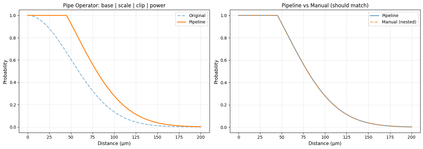
⛓️ Pipe operator benefits:
  ✓ More readable (left-to-right flow)
  ✓ Easier to modify pipeline
  ✓ Composable and modular

  Pipeline ≈ Manual: True
Complex Composition Example#
# Build a complex connectivity pattern
# Goal: Strong local, weak intermediate, moderate long-range

local_excitation = init.GaussianProfile(sigma=30.0 * u.um)
intermediate_inhibition = init.GaussianProfile(sigma=80.0 * u.um)
long_range_excitation = init.GaussianProfile(sigma=150.0 * u.um)

# Compose with weights
complex_pattern = (
    local_excitation * 1.0
    - intermediate_inhibition * 0.3
    + long_range_excitation * 0.2
).clip(min_val=0.0, max_val=1.0)

# Visualize
fig = plt.figure(figsize=(14, 10))
gs = GridSpec(3, 2, figure=fig)

distances = np.linspace(0, 300, 500) * u.um

# Components
ax1 = fig.add_subplot(gs[0, :])
ax1.plot(distances.mantissa, local_excitation.probability(distances),
         label='Local excitation', linewidth=2)
ax1.plot(distances.mantissa, intermediate_inhibition.probability(distances) * 0.3,
         label='Intermediate inhibition × 0.3', linewidth=2)
ax1.plot(distances.mantissa, long_range_excitation.probability(distances) * 0.2,
         label='Long-range excitation × 0.2', linewidth=2)
ax1.set_xlabel('Distance (μm)')
ax1.set_ylabel('Component strength')
ax1.set_title('Individual Components')
ax1.legend()
ax1.grid(alpha=0.3)

# Composed pattern
ax2 = fig.add_subplot(gs[1, :])
prob_complex = complex_pattern.probability(distances)
ax2.plot(distances.mantissa, prob_complex, linewidth=3, color='purple')
ax2.fill_between(distances.mantissa, prob_complex, alpha=0.3, color='purple')
ax2.axhline(0, color='black', linestyle='-', linewidth=0.5)
ax2.set_xlabel('Distance (μm)')
ax2.set_ylabel('Connection Probability')
ax2.set_title('Complex Composed Pattern (clipped to [0, 1])')
ax2.grid(alpha=0.3)

# 2D visualization
ax3 = fig.add_subplot(gs[2, 0])
x = np.linspace(-150, 150, 100)
y = np.linspace(-150, 150, 100)
X, Y = np.meshgrid(x, y)
D = np.sqrt(X**2 + Y**2) * u.um
P = complex_pattern.probability(D)
im = ax3.imshow(P, extent=[-150, 150, -150, 150], origin='lower', cmap='RdYlBu_r')
ax3.set_xlabel('X position (μm)')
ax3.set_ylabel('Y position (μm)')
ax3.set_title('2D Spatial Pattern')
plt.colorbar(im, ax=ax3, label='Probability')

# Cross-section
ax4 = fig.add_subplot(gs[2, 1])
center_row = P[50, :]
ax4.plot(x, center_row, linewidth=2)
ax4.fill_between(x, center_row, alpha=0.3)
ax4.set_xlabel('Distance from center (μm)')
ax4.set_ylabel('Connection Probability')
ax4.set_title('Cross-section Through Center')
ax4.grid(alpha=0.3)

plt.suptitle('Complex Multi-Scale Connectivity Pattern', fontsize=14, y=0.995)
plt.tight_layout()
plt.show()

print("\n🧠 This pattern creates:")
print("  1. Strong local excitation (0-50 μm)")
print("  2. Lateral inhibition (50-150 μm)")
print("  3. Weak long-range excitation (150-300 μm)")
print("\n  Common in cortical circuits!")
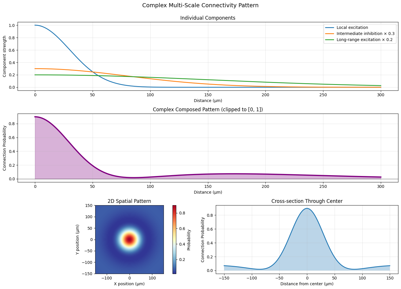
🧠 This pattern creates:
  1. Strong local excitation (0-50 μm)
  2. Lateral inhibition (50-150 μm)
  3. Weak long-range excitation (150-300 μm)

  Common in cortical circuits!
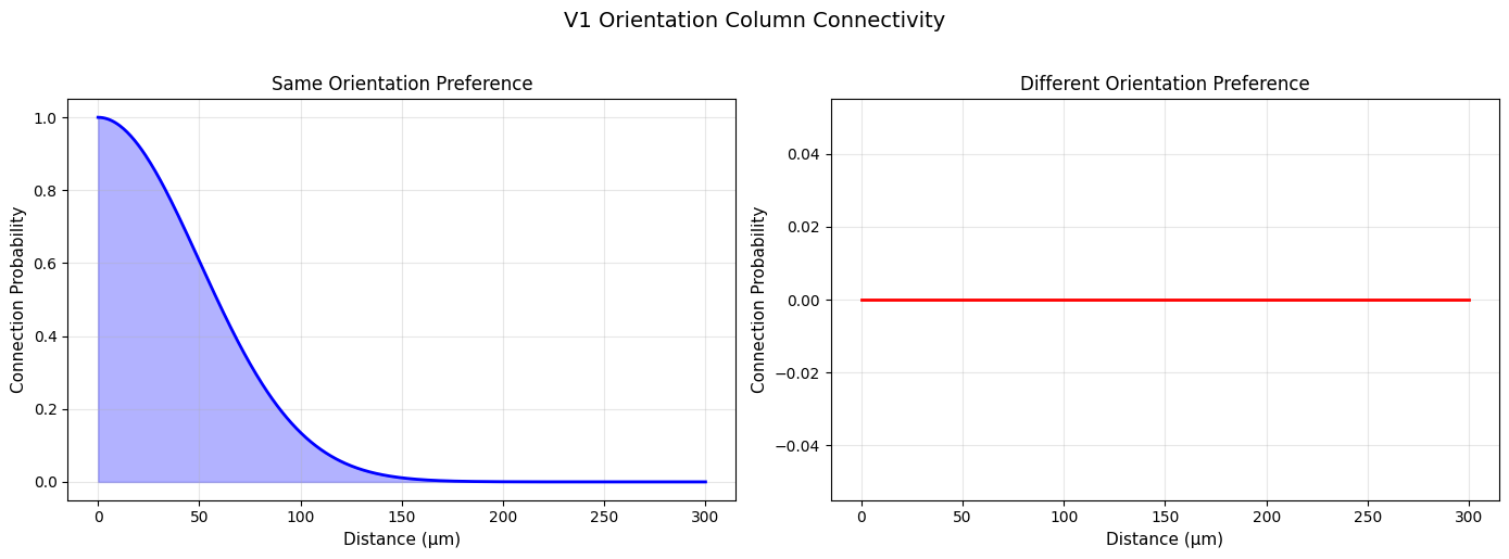
5. Real-World Neuroscience Applications#
Application 1: V1 Orientation Columns#
# Model V1 orientation column connectivity
# Same orientation: strong local connection
# Different orientation: lateral inhibition

# Simplified: distance-based approximation
same_orientation = init.GaussianProfile(sigma=50.0 * u.um)
different_orientation = (
    init.DoGProfile(
        sigma_center=40.0 * u.um,
        sigma_surround=100.0 * u.um,
        amplitude_center=0.3,
        amplitude_surround=0.4
    )
).clip(min_val=0.0)

fig, axes = plt.subplots(1, 2, figsize=(14, 5))

distances = np.linspace(0, 300, 500) * u.um

# Same orientation
prob_same = same_orientation.probability(distances)
axes[0].plot(distances.mantissa, prob_same, linewidth=2, color='blue')
axes[0].fill_between(distances.mantissa, prob_same, alpha=0.3, color='blue')
axes[0].set_xlabel('Distance (μm)', fontsize=11)
axes[0].set_ylabel('Connection Probability', fontsize=11)
axes[0].set_title('Same Orientation Preference', fontsize=12)
axes[0].grid(alpha=0.3)

# Different orientation
prob_diff = different_orientation.probability(distances)
axes[1].plot(distances.mantissa, prob_diff, linewidth=2, color='red')
axes[1].fill_between(distances.mantissa, prob_diff, alpha=0.3, color='red')
axes[1].set_xlabel('Distance (μm)', fontsize=11)
axes[1].set_ylabel('Connection Probability', fontsize=11)
axes[1].set_title('Different Orientation Preference', fontsize=12)
axes[1].grid(alpha=0.3)

plt.suptitle('V1 Orientation Column Connectivity', fontsize=14, y=1.02)
plt.tight_layout()
plt.show()

print("\n👁️ V1 orientation columns:")
print("  - Neurons preferring same orientation connect strongly locally")
print("  - Neurons with different orientations show lateral inhibition")
print("  - Creates orientation selectivity sharpening")
👁️ V1 orientation columns:
  - Neurons preferring same orientation connect strongly locally
  - Neurons with different orientations show lateral inhibition
  - Creates orientation selectivity sharpening
Application 2: Hippocampal Place Cells#
# Hippocampal place cell connectivity
# Overlapping place fields → stronger connection

def place_field_overlap(distance, field_size=40.0):
    """
    Model place field overlap as function of cell distance.
    """
    # Simplified: Gaussian overlap
    profile = init.GaussianProfile(sigma=field_size * u.cm)
    return profile.probability(distance)

# CA3 recurrent connections: bimodal (local + long-range)
ca3_recurrent = init.BimodalProfile(
    sigma1=50.0 * u.um,
    sigma2=200.0 * u.um,
    center1=0.0 * u.um,
    center2=300.0 * u.um,
    amplitude1=0.8,
    amplitude2=0.3
)

# CA1 connections: more local
ca1_local = init.GaussianProfile(sigma=80.0 * u.um)

fig, axes = plt.subplots(1, 2, figsize=(14, 5))

distances = np.linspace(0, 500, 500) * u.um

# CA3 recurrent
prob_ca3 = ca3_recurrent.probability(distances)
axes[0].plot(distances.mantissa, prob_ca3, linewidth=2)
axes[0].fill_between(distances.mantissa, prob_ca3, alpha=0.3)
axes[0].set_xlabel('Distance (μm)', fontsize=11)
axes[0].set_ylabel('Connection Probability', fontsize=11)
axes[0].set_title('CA3 Recurrent Connectivity', fontsize=12)
axes[0].grid(alpha=0.3)

# CA1 local
prob_ca1 = ca1_local.probability(distances)
axes[1].plot(distances.mantissa, prob_ca1, linewidth=2, color='orange')
axes[1].fill_between(distances.mantissa, prob_ca1, alpha=0.3, color='orange')
axes[1].set_xlabel('Distance (μm)', fontsize=11)
axes[1].set_ylabel('Connection Probability', fontsize=11)
axes[1].set_title('CA1 Local Connectivity', fontsize=12)
axes[1].grid(alpha=0.3)

plt.suptitle('Hippocampal Connectivity Patterns', fontsize=14, y=1.02)
plt.tight_layout()
plt.show()

print("\n🧠 Hippocampal connectivity:")
print("  CA3: Bimodal (supports pattern completion)")
print("  CA1: More local (different computational role)")
print("  Place cells with overlapping fields connect preferentially")
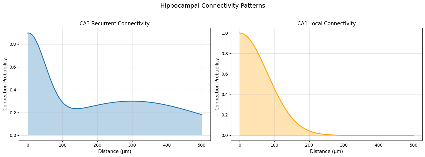
🧠 Hippocampal connectivity:
  CA3: Bimodal (supports pattern completion)
  CA1: More local (different computational role)
  Place cells with overlapping fields connect preferentially
Application 3: Cortical Layer-Specific Connectivity#
# Different cortical layers have different connectivity patterns

# Layer 2/3: Local horizontal connections
layer23 = init.GaussianProfile(sigma=200.0 * u.um)

# Layer 4: Dense local connections
layer4 = init.GaussianProfile(sigma=100.0 * u.um)

# Layer 5: Long-range projections
layer5 = init.BimodalProfile(
    sigma1=100.0 * u.um,
    sigma2=400.0 * u.um,
    center1=0.0 * u.um,
    center2=600.0 * u.um,
    amplitude1=0.7,
    amplitude2=0.4
)

# Layer 6: Feedback connections
layer6 = init.ExponentialProfile(decay_constant=300.0 * u.um)

# Visualize
fig, axes = plt.subplots(2, 2, figsize=(14, 10))
axes = axes.flatten()

distances = np.linspace(0, 800, 500) * u.um

layers = [
    (layer23, 'Layer 2/3: Horizontal Connections', 'blue'),
    (layer4, 'Layer 4: Dense Local', 'green'),
    (layer5, 'Layer 5: Long-range Projections', 'red'),
    (layer6, 'Layer 6: Feedback', 'purple'),
]

for ax, (profile, title, color) in zip(axes, layers):
    prob = profile.probability(distances)
    ax.plot(distances.mantissa, prob, linewidth=2, color=color)
    ax.fill_between(distances.mantissa, prob, alpha=0.3, color=color)
    ax.set_xlabel('Distance (μm)', fontsize=11)
    ax.set_ylabel('Connection Probability', fontsize=11)
    ax.set_title(title, fontsize=12)
    ax.grid(alpha=0.3)

plt.suptitle('Layer-Specific Cortical Connectivity', fontsize=14, y=1.00)
plt.tight_layout()
plt.show()

print("\n📊 Layer-specific properties:")
print("  L2/3: Broad horizontal connections (integrate information)")
print("  L4: Dense local (receive thalamic input)")
print("  L5: Long-range projections (output layer)")
print("  L6: Feedback to thalamus (modulation)")
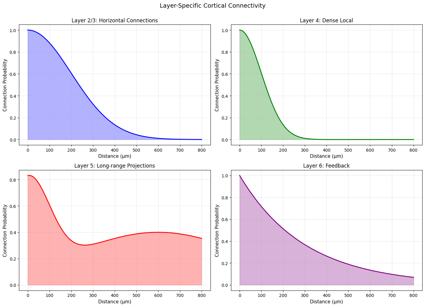
📊 Layer-specific properties:
  L2/3: Broad horizontal connections (integrate information)
  L4: Dense local (receive thalamic input)
  L5: Long-range projections (output layer)
  L6: Feedback to thalamus (modulation)
Summary#
In this tutorial, we covered:
Basic profiles: Gaussian, Exponential, PowerLaw, Linear, Step
Advanced profiles: Sigmoid, DoG, Logistic, Bimodal, MexicanHat
Profile composition: Arithmetic operations, clipping, transformations
Pipe operator: Functional composition for clean code
Real applications: V1, hippocampus, cortical layers
Profile Selection Guide:#
Pattern |
Profile |
|---|---|
Local excitation |
Gaussian |
Long-range decay |
Exponential |
Scale-free |
PowerLaw |
Hard boundary |
Step, Linear |
Smooth transition |
Sigmoid, Logistic |
Lateral inhibition |
DoG, MexicanHat |
Multi-scale |
Bimodal, Composed |