

The Functional API#
Each functional generator returns an array of length \(\lceil T/dt \rceil\) (or shape (steps, n) for n independent channels). This tutorial goes through all of them, grouped by family, and checks each against what its parameters promise.
Family |
Functions |
|---|---|
Piecewise |
|
Periodic |
|
Pulses |
|
Stochastic |
|
The composable classes take the same parameters, but some are in a different positional order (for example spike(sp_times, sp_lens, sp_sizes, duration) versus Spike(sp_times, duration, sp_lens, sp_sizes)). Passing parameters by keyword avoids mistakes when switching between the two.
1. Setup#
import brainstate
import brainunit as u
import matplotlib.pyplot as plt
import numpy as np
from scipy import signal as sps

import braintools.input as inp

brainstate.environ.set(dt=0.1 * u.ms)
dt_ms = 0.1


def t_of(x):
    return np.arange(len(x)) * dt_ms


def show(panels, ncols=2, height=2.2):
    # Plot a dict {title: array} on a grid.
    nrows = int(np.ceil(len(panels) / ncols))
    fig, axes = plt.subplots(nrows, ncols, figsize=(6 * ncols, height * nrows), squeeze=False)
    for ax, (title, x) in zip(axes.flat, panels.items()):
        ax.plot(t_of(x), u.get_mantissa(x), lw=1)
        ax.set_title(title, fontsize=10)
    for ax in axes.flat[len(panels):]:
        ax.axis("off")
    for ax in axes[-1]:
        ax.set_xlabel("time (ms)")
    fig.tight_layout()
    plt.show()
2. Piecewise Signals#
section(values, durations)concatenates constant segments; each value lasts for its duration.constant([(value, duration), ...])does the same from pairs, and returns a tuple(array, total_duration).step(amplitudes, step_times, duration)sets each amplitude from its start time until the next start time. Times are sorted first.ramp(c_start, c_end, duration, t_start=None, t_end=None)goes linearly fromc_starttoc_endbetweent_startandt_endand is 0 outside that window.
sec = inp.section([0, 1, 0.5, 0] * u.nA, [20, 30, 30, 20] * u.ms)
const, total = inp.constant([(0 * u.nA, 20 * u.ms), (1 * u.nA, 30 * u.ms), (0.5 * u.nA, 30 * u.ms), (0 * u.nA, 20 * u.ms)])
stp = inp.step([0, 1, 0.5, 0] * u.nA, [0, 20, 50, 80] * u.ms, duration=100 * u.ms)
rmp = inp.ramp(0 * u.nA, 1 * u.nA, 100 * u.ms, t_start=20 * u.ms, t_end=80 * u.ms)

print("constant returns total duration:", total)
print("section == constant == step:", bool(u.math.allclose(sec, const)) and bool(u.math.allclose(sec, stp)))
print(f"ramp is 0 before 20 ms: {float(rmp[199].to_decimal(u.nA)) == 0.0}, "
      f"reaches {float(rmp[799].to_decimal(u.nA)):.3f} nA at 80 ms, then 0: {float(rmp[800].to_decimal(u.nA)) == 0.0}")
show({"section / constant / step": sec, "ramp(0, 1 nA, t_start=20, t_end=80)": rmp})
constant returns total duration: 100 ms
section == constant == step: True
ramp is 0 before 20 ms: True, reaches 1.000 nA at 80 ms, then 0: True

3. Periodic Signals#
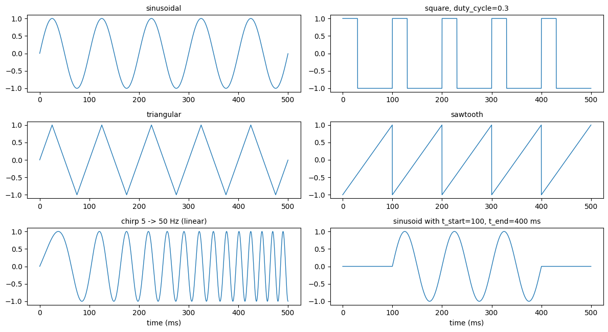
All periodic generators take amplitude, frequency, and duration, and optionally t_start / t_end (the signal is 0 outside the window and starts at phase 0 at t_start).
sinusoidal,square,triangular,sawtoothoscillate between-amplitudeand+amplitude;squarehas aduty_cycle(fraction of each period at+amplitude).bias=Trueaddsamplitude, so the signal runs from 0 to2 * amplitude.chirp(amplitude, f_start, f_end, duration, method='linear' | 'logarithmic')sweeps the frequency.noisy_sinusoidal(amplitude, frequency, noise_amplitude, duration, seed=...)adds independent Gaussian noise with standard deviationnoise_amplitudeto every sample.
The checks below measure the frequency from rising zero crossings and compare the chirp with scipy.signal.chirp.
def measured_frequency(x):
    y = np.asarray(x) - np.mean(x)
    up = np.flatnonzero((y[:-1] < 0) & (y[1:] >= 0))
    return (len(up) - 1) / ((up[-1] - up[0]) * dt_ms * 1e-3)


periodic = {
    "sinusoidal": inp.sinusoidal(1.0, 10 * u.Hz, 500 * u.ms),
    "square, duty_cycle=0.3": inp.square(1.0, 10 * u.Hz, 500 * u.ms, duty_cycle=0.3),
    "triangular": inp.triangular(1.0, 10 * u.Hz, 500 * u.ms),
    "sawtooth": inp.sawtooth(1.0, 10 * u.Hz, 500 * u.ms),
}
for name, x in periodic.items():
    print(f"{name:24s} frequency {measured_frequency(x):6.2f} Hz, range [{x.min():.2f}, {x.max():.2f}]")
sq = periodic["square, duty_cycle=0.3"]
print(f"square fraction of time high: {np.mean(sq > 0):.3f}")
biased = inp.sinusoidal(1.0, 10 * u.Hz, 500 * u.ms, bias=True)
print(f"bias=True range: [{biased.min():.2f}, {biased.max():.2f}]")

t_sec = np.arange(10000) * dt_ms * 1e-3
for method in ["linear", "logarithmic"]:
    ch = np.asarray(inp.chirp(1.0, 5 * u.Hz, 50 * u.Hz, 1000 * u.ms, method=method))
    ref = sps.chirp(t_sec, 5, 1.0, 50, method=method, phi=-90)  # phi=-90 turns scipy's cosine into a sine
    print(f"chirp {method:11s} max |difference| from scipy: {np.abs(ch - ref).max():.1e}")

noisy = inp.noisy_sinusoidal(1.0, 10 * u.Hz, 0.3, 500 * u.ms, seed=0)
print(f"noisy_sinusoidal residual std: {np.std(noisy - periodic['sinusoidal']):.3f} (noise_amplitude 0.3)")

show({**periodic,
      "chirp 5 -> 50 Hz (linear)": inp.chirp(1.0, 5 * u.Hz, 50 * u.Hz, 500 * u.ms),
      "sinusoid with t_start=100, t_end=400 ms": inp.sinusoidal(1.0, 10 * u.Hz, 500 * u.ms, t_start=100 * u.ms, t_end=400 * u.ms)})
sinusoidal               frequency  10.00 Hz, range [-1.00, 1.00]
square, duty_cycle=0.3   frequency  10.00 Hz, range [-1.00, 1.00]
triangular               frequency  10.00 Hz, range [-1.00, 1.00]
sawtooth                 frequency  10.00 Hz, range [-1.00, 1.00]
square fraction of time high: 0.300
bias=True range: [0.00, 2.00]
chirp linear      max |difference| from scipy: 3.0e-08
chirp logarithmic max |difference| from scipy: 3.0e-08
noisy_sinusoidal residual std: 0.296 (noise_amplitude 0.3)
4. Pulses#
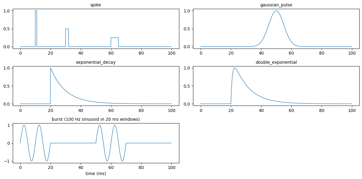
spike(sp_times, sp_lens, sp_sizes, duration): rectangular pulses starting atsp_times;sp_lensandsp_sizesmay be a single value or one per pulse.gaussian_pulse(amplitude, center, sigma, duration): peak valueamplitudeatcenter.exponential_decay(amplitude, tau, duration, t_start=None): jumps toamplitudeatt_startand decays as \(e^{-(t - t_{start})/\tau}\).double_exponential(amplitude, tau_rise, tau_decay, duration, t_start=None): the difference of two exponentials, normalized so its peak equalsamplitude; the peak occurs \(\frac{\tau_r \tau_d}{\tau_d - \tau_r}\ln\frac{\tau_d}{\tau_r}\) aftert_start.burst(burst_amp, burst_freq, burst_duration, inter_burst_interval, n_bursts, duration):n_burstswindows of lengthburst_duration, separated byinter_burst_interval, each filled with a sinusoid of frequencyburst_freqthat starts at phase 0. For a train of rectangular pulses usespikeorsquareinstead.
spk = inp.spike(sp_times=[10, 30, 60] * u.ms, sp_lens=[1, 2, 5] * u.ms, sp_sizes=[1.0, 0.5, 0.25], duration=100 * u.ms)
gau = inp.gaussian_pulse(1.0, center=50 * u.ms, sigma=5 * u.ms, duration=100 * u.ms)
exd = inp.exponential_decay(1.0, tau=10 * u.ms, duration=100 * u.ms, t_start=20 * u.ms)
dex = inp.double_exponential(1.0, tau_rise=1 * u.ms, tau_decay=10 * u.ms, duration=100 * u.ms, t_start=20 * u.ms)
bur = inp.burst(burst_amp=1.0, burst_freq=100 * u.Hz, burst_duration=20 * u.ms,
                inter_burst_interval=30 * u.ms, n_bursts=2, duration=100 * u.ms)

print("spike pulse widths (samples):", [int(np.sum(np.asarray(spk) == v)) for v in (1.0, 0.5, 0.25)])
print(f"gaussian peak {gau.max():.3f} at {t_of(gau)[np.argmax(gau)]:.1f} ms")
print(f"exponential_decay at t_start + tau: {exd[300]:.4f} (exp(-1) = {np.exp(-1):.4f})")
t_peak = 1 * 10 / (10 - 1) * np.log(10 / 1)
print(f"double_exponential peak {dex.max():.3f} at {t_of(dex)[np.argmax(dex)] - 20:.1f} ms after onset (theory {t_peak:.2f} ms)")
on = np.flatnonzero(np.abs(np.asarray(bur)) > 0) * dt_ms
print(f"burst is non-zero between {on[0]:.1f} and {on[-1]:.1f} ms (bursts at 0-20 and 50-70 ms)")

show({"spike": spk, "gaussian_pulse": gau, "exponential_decay": exd,
      "double_exponential": dex, "burst (100 Hz sinusoid in 20 ms windows)": bur}, height=2.0)
spike pulse widths (samples): [10, 20, 50]
gaussian peak 1.000 at 50.0 ms
exponential_decay at t_start + tau: 0.3679 (exp(-1) = 0.3679)
double_exponential peak 1.000 at 2.6 ms after onset (theory 2.56 ms)
burst is non-zero between 0.1 and 69.9 ms (bursts at 0-20 and 50-70 ms)
5. Stochastic Processes#
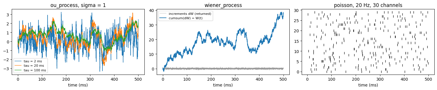
All three accept seed for reproducibility and n for independent channels (output shape (steps, n)).
ou_process(mean, sigma, tau, duration): an Ornstein-Uhlenbeck process, i.e. noise with correlation timetau. It starts atmean, andsigmais its stationary standard deviation; the autocorrelation decays as \(e^{-|\text{lag}|/\tau}\). The update is exact, so the statistics do not depend ondtor on the time unit.wiener_process(duration, sigma): the increments \(dW \sim \mathcal N(0, \sigma^2 dt)\) of a Wiener process, one independent sample per step. This is white noise, not the Brownian path \(W(t)\) (usecumsumfor the path).dtenters as its number in the unit it was set with, so keep the time unit consistent when choosingsigma.poisson(rate, duration, amplitude=1): in each step an event occurs with probabilityrate * dt, and the output isamplitudeon event steps and 0 elsewhere.
ou = np.asarray(inp.ou_process(mean=0.5, sigma=0.2, tau=10 * u.ms, duration=20_000 * u.ms, n=8, seed=0))
x = ou[2000:] - ou[2000:].mean(axis=0)
lag = 100  # 10 ms
rho = np.mean(x[:-lag] * x[lag:], axis=0) / np.var(x, axis=0)
print(f"OU (8 channels): mean {ou.mean():.3f} (0.5), std {ou.std(axis=0).mean():.3f} (0.2), "
      f"autocorrelation at lag tau {rho.mean():.3f} (exp(-1) = {np.exp(-1):.3f})")

dw = inp.wiener_process(duration=20_000 * u.ms, sigma=2.0, seed=0)
print(f"Wiener increments: std {np.std(dw):.4f} (sigma*sqrt(dt) = {2.0 * np.sqrt(dt_ms):.4f}), "
      f"lag-1 correlation {np.corrcoef(dw[:-1], dw[1:])[0, 1]:+.3f}")

pois = inp.poisson(rate=20 * u.Hz, duration=1000 * u.ms, n=200, seed=0)
counts = np.asarray(pois).sum(axis=0)
event_times = [np.flatnonzero(col) * dt_ms for col in np.asarray(pois).T]
isis = np.concatenate([np.diff(e) for e in event_times])
print(f"Poisson 20 Hz over 1 s, 200 channels: mean count {counts.mean():.2f} (20), "
      f"Fano factor {counts.var() / counts.mean():.2f} (1), ISI CV {isis.std() / isis.mean():.2f} (1)")
OU (8 channels): mean 0.503 (0.5), std 0.199 (0.2), autocorrelation at lag tau 0.367 (exp(-1) = 0.368)
Wiener increments: std 0.6312 (sigma*sqrt(dt) = 0.6325), lag-1 correlation -0.001
Poisson 20 Hz over 1 s, 200 channels: mean count 19.97 (20), Fano factor 1.03 (1), ISI CV 1.00 (1)
The OU std, the Wiener increment std, and the Poisson statistics all match their definitions. The figure shows OU processes with different correlation times (same seed), a Wiener increment trace with its cumulative path, and a Poisson raster.
fig, axes = plt.subplots(1, 3, figsize=(15, 3.2))
for tau in [2, 20, 100]:
    trace = inp.ou_process(mean=0.0, sigma=1.0, tau=tau * u.ms, duration=500 * u.ms, seed=1)
    axes[0].plot(t_of(trace), trace, lw=1, label=f"tau = {tau} ms")
axes[0].set_title("ou_process, sigma = 1")
axes[0].legend(fontsize=8)

dw = inp.wiener_process(duration=500 * u.ms, sigma=1.0, seed=1)
axes[1].plot(t_of(dw), dw, lw=0.5, color="0.6", label="increments dW (returned)")
axes[1].plot(t_of(dw), np.cumsum(dw), lw=1.5, label="cumsum(dW) = W(t)")
axes[1].set_title("wiener_process")
axes[1].legend(fontsize=8)

raster = np.asarray(inp.poisson(rate=20 * u.Hz, duration=500 * u.ms, n=30, seed=2))
rows, cols = np.nonzero(raster.T)
axes[2].plot(cols * dt_ms, rows, "|", ms=6, color="k")
axes[2].set_title("poisson, 20 Hz, 30 channels")
for ax in axes:
    ax.set_xlabel("time (ms)")
fig.tight_layout()
plt.show()
6. Assembling a Protocol from Arrays#
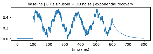
Functional outputs are ordinary arrays, so a protocol can be assembled with u.math.concatenate (segments one after another) and + (overlays of equal length). The composable API in the next tutorial does the same with less bookkeeping.
baseline = inp.section([0] * u.nA, [100 * u.ms])
drive = inp.sinusoidal(0.2 * u.nA, 8 * u.Hz, 500 * u.ms) + inp.ou_process(0.3 * u.nA, 0.05 * u.nA, 5 * u.ms, 500 * u.ms, seed=0)
recovery = inp.exponential_decay(0.3 * u.nA, tau=50 * u.ms, duration=200 * u.ms)

protocol = u.math.concatenate([baseline, drive, recovery])
print(f"{protocol.shape[0]} samples = {protocol.shape[0] * dt_ms:.0f} ms, unit {u.get_unit(protocol)}")
show({"baseline | 8 Hz sinusoid + OU noise | exponential recovery": protocol}, ncols=1)
8000 samples = 800 ms, unit nA
Summary#
Piecewise:
sectionandconstanttake durations,steptakes start times,ramptakes a window.Periodic generators share
amplitude,frequency,t_start/t_end, andbias;chirpmatchesscipy.signal.chirp.double_exponentialis peak-normalized;burstfills its windows with a sinusoid.ou_process(sigma=...)sets the stationary standard deviation;wiener_processreturns increments with std \(\sigma\sqrt{dt}\);poissonplaces events with probabilityrate * dtper step.Use keyword arguments: several functional and composable signatures order their parameters differently.