Tutorial 4: Composite and Distance-Modulated Initialization Strategies

Tutorial 4: Composite and Distance-Modulated Initialization Strategies#

This tutorial explores advanced initialization strategies that combine multiple distributions and modulate weights based on spatial distance. These techniques enable the creation of biologically realistic and heterogeneous neural networks.

Topics Covered#

Composite initialization patterns
Mixture distributions for heterogeneous populations
Conditional initialization based on neuron properties
Scaled and Clipped distributions
DistanceModulated: combining base distributions with distance profiles
Building complex initialization schemes
Integration example: biologically realistic connectivity patterns

Installation and Setup#

# Install braintools if needed
# !pip install braintools brainunit matplotlib numpy scipy

import numpy as np
import matplotlib.pyplot as plt
from matplotlib.gridspec import GridSpec
import brainunit as u
from braintools import init

# Set random seed for reproducibility
np.random.seed(42)

# Configure matplotlib
plt.rcParams['figure.figsize'] = (12, 4)
plt.rcParams['font.size'] = 10

1. Introduction to Composite Initialization#

Why Composite Initialization?#

Real neural networks exhibit:

Heterogeneity: Not all neurons/connections are identical
Population diversity: Excitatory vs inhibitory, different subtypes
Spatial structure: Distance-dependent properties
Complex patterns: Multiple mechanisms combine

Types of Composition#

Mixture: Random selection from multiple distributions
Conditional: Different distributions based on properties
Scaled/Clipped: Transform a base distribution
Distance-modulated: Spatial modulation of weights

Key Principles#

Modularity: Build complex from simple components
Biological realism: Match observed data
Composability: Combine multiple strategies

2. Mixture Distributions#

Mixture distributions randomly select from multiple distributions according to specified weights. This creates heterogeneous populations.

Mathematical Definition#

For distributions \(D_1, D_2, \ldots, D_k\) with weights \(w_1, w_2, \ldots, w_k\) (where \(\sum w_i = 1\)):

\[W \sim \sum_{i=1}^k w_i D_i\]

Use Cases#

Multiple synapse types
Heterogeneous connection strengths
Multimodal weight distributions
Subpopulation diversity

# Example 1: Two-component mixture (weak and strong synapses)
mixture_simple = init.Mixture(
    distributions=[
        init.Normal(mean=0.3 * u.nS, std=0.05 * u.nS),  # Weak synapses
        init.Normal(mean=1.2 * u.nS, std=0.2 * u.nS),   # Strong synapses
    ],
    weights=[0.7, 0.3]  # 70% weak, 30% strong
)

# Generate samples
rng = np.random.default_rng(42)
weights_mixture = mixture_simple(2000, rng=rng)

# For comparison: single normal distribution
weights_single = init.Normal(0.6 * u.nS, 0.4 * u.nS)(2000, rng=rng)

# Visualize
fig, axes = plt.subplots(1, 2, figsize=(14, 5))

# Mixture distribution
axes[0].hist(weights_mixture.mantissa, bins=50, alpha=0.7, edgecolor='black', density=True)
axes[0].axvline(0.3, color='blue', linestyle='--', alpha=0.7, label='Weak peak (0.3 nS)')
axes[0].axvline(1.2, color='red', linestyle='--', alpha=0.7, label='Strong peak (1.2 nS)')
axes[0].set_xlabel(f'Conductance ({weights_mixture.unit})', fontsize=11)
axes[0].set_ylabel('Density', fontsize=11)
axes[0].set_title('Mixture: Bimodal Distribution', fontsize=12)
axes[0].legend()
axes[0].grid(alpha=0.3)

# Single distribution for comparison
axes[1].hist(weights_single.mantissa, bins=50, alpha=0.7, edgecolor='black', 
             density=True, color='gray')
axes[1].set_xlabel(f'Conductance ({weights_single.unit})', fontsize=11)
axes[1].set_ylabel('Density', fontsize=11)
axes[1].set_title('Single: Unimodal Distribution', fontsize=12)
axes[1].grid(alpha=0.3)

plt.tight_layout()
plt.show()

print(f"Mixture Distribution:")
print(f"  Mean: {weights_mixture.mean():.3f}")
print(f"  Std: {weights_mixture.std():.3f}")
print(f"  Range: [{weights_mixture.min():.2f}, {weights_mixture.max():.2f}]")
print(f"\nSingle Distribution:")
print(f"  Mean: {weights_single.mean():.3f}")
print(f"  Std: {weights_single.std():.3f}")
print(f"  Range: [{weights_single.min():.2f}, {weights_single.max():.2f}]")

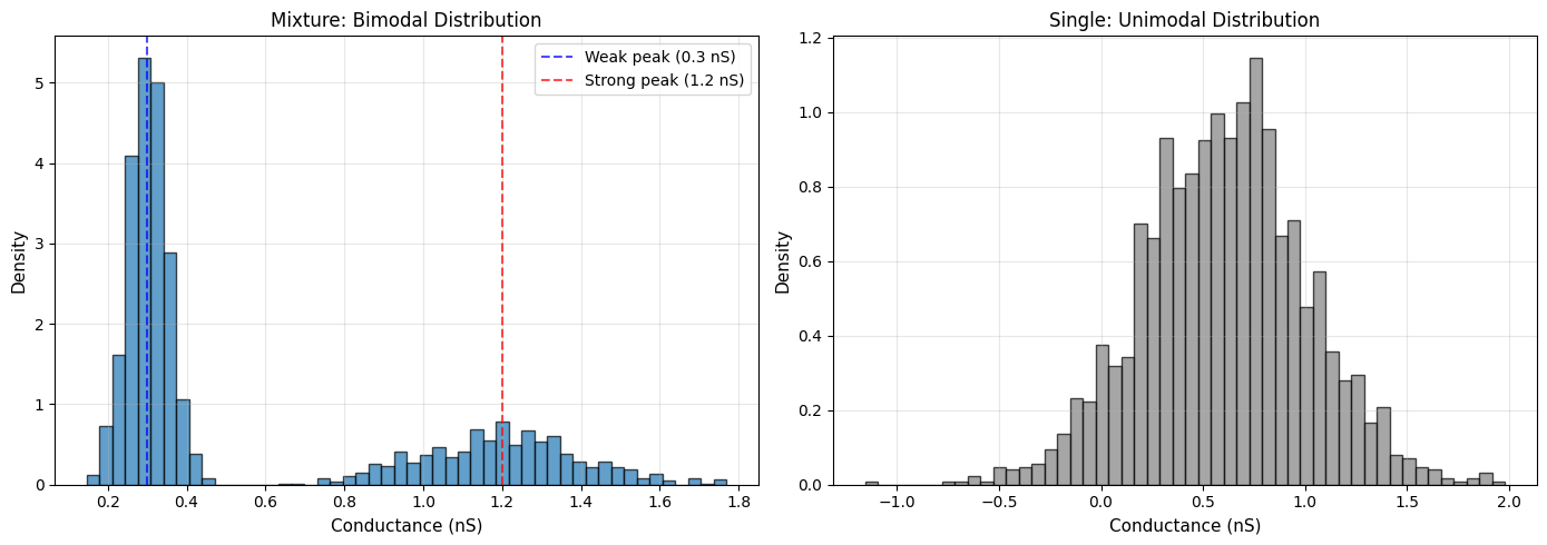
../_images/5c9be12376a7fab6ef9208092c4f422fc9378a1aed4502b1813776edbab37b7a.png

Mixture Distribution:
  Mean: 0.579 * nsiemens
  Std: 0.431 * nsiemens
  Range: [0.15 * nsiemens, 1.77 * nsiemens]

Single Distribution:
  Mean: 0.604 * nsiemens
  Std: 0.403 * nsiemens
  Range: [-1.16 * nsiemens, 1.98 * nsiemens]

Multi-Component Mixture#

# Example 2: Three-component mixture (weak, medium, strong)
mixture_triple = init.Mixture(
    distributions=[
        init.Normal(mean=0.2 * u.nS, std=0.03 * u.nS),   # Weak
        init.Normal(mean=0.6 * u.nS, std=0.08 * u.nS),   # Medium
        init.Normal(mean=1.5 * u.nS, std=0.25 * u.nS),   # Strong
    ],
    weights=[0.5, 0.35, 0.15]  # 50% weak, 35% medium, 15% strong
)

weights_triple = mixture_triple(3000, rng=rng)

# Visualize
fig, axes = plt.subplots(1, 2, figsize=(14, 5))

# Histogram
axes[0].hist(weights_triple.mantissa, bins=60, alpha=0.7, edgecolor='black', density=True)
axes[0].axvline(0.2, color='blue', linestyle='--', alpha=0.5, label='Weak (50%)')
axes[0].axvline(0.6, color='green', linestyle='--', alpha=0.5, label='Medium (35%)')
axes[0].axvline(1.5, color='red', linestyle='--', alpha=0.5, label='Strong (15%)')
axes[0].set_xlabel(f'Conductance ({weights_triple.unit})', fontsize=11)
axes[0].set_ylabel('Density', fontsize=11)
axes[0].set_title('Three-Component Mixture', fontsize=12)
axes[0].legend()
axes[0].grid(alpha=0.3)

# Scatter plot showing heterogeneity
indices = np.arange(len(weights_triple))[:300]  # Show first 300
colors = weights_triple.mantissa[:300]
scatter = axes[1].scatter(indices, weights_triple.mantissa[:300], 
                          c=colors, cmap='viridis', s=30, alpha=0.6)
axes[1].axhline(0.2, color='blue', linestyle='--', alpha=0.3)
axes[1].axhline(0.6, color='green', linestyle='--', alpha=0.3)
axes[1].axhline(1.5, color='red', linestyle='--', alpha=0.3)
axes[1].set_xlabel('Connection index', fontsize=11)
axes[1].set_ylabel(f'Conductance ({weights_triple.unit})', fontsize=11)
axes[1].set_title('Weight Heterogeneity (first 300)', fontsize=12)
plt.colorbar(scatter, ax=axes[1], label='Conductance (nS)')
axes[1].grid(alpha=0.3)

plt.tight_layout()
plt.show()

# Classify synapses
weak_mask = weights_triple.mantissa < 0.4
strong_mask = weights_triple.mantissa > 1.0
medium_mask = ~weak_mask & ~strong_mask

print(f"\nSynapse classification:")
print(f"  Weak (< 0.4 nS): {np.sum(weak_mask)} ({100*np.sum(weak_mask)/len(weights_triple):.1f}%)")
print(f"  Medium (0.4-1.0 nS): {np.sum(medium_mask)} ({100*np.sum(medium_mask)/len(weights_triple):.1f}%)")
print(f"  Strong (> 1.0 nS): {np.sum(strong_mask)} ({100*np.sum(strong_mask)/len(weights_triple):.1f}%)")

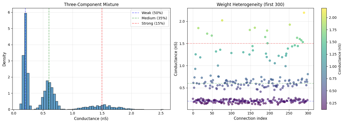
../_images/0425e8b8a4b0a2e4a661784e79ca9ff30e0d3d71a9002e7b1290a90f910acc03.png

Synapse classification:
  Weak (< 0.4 nS): 1483 (49.4%)
  Medium (0.4-1.0 nS): 1075 (35.8%)
  Strong (> 1.0 nS): 442 (14.7%)

Mixture with Different Distribution Types#

# Mix different distribution types
mixture_mixed = init.Mixture(
    distributions=[
        init.Normal(mean=0.5 * u.nS, std=0.1 * u.nS),     # Normal
        init.LogNormal(mean=0.8 * u.nS, std=0.3 * u.nS),  # LogNormal
        init.Gamma(shape=3.0, scale=0.2 * u.nS),          # Gamma
    ],
    weights=[0.5, 0.3, 0.2]
)

weights_mixed = mixture_mixed(3000, rng=rng)

# Visualize
fig, ax = plt.subplots(1, 1, figsize=(10, 5))

ax.hist(weights_mixed.mantissa, bins=60, alpha=0.7, edgecolor='black', density=True)
ax.set_xlabel(f'Conductance ({weights_mixed.unit})', fontsize=11)
ax.set_ylabel('Density', fontsize=11)
ax.set_title('Mixture of Different Distribution Types\n(Normal + LogNormal + Gamma)', fontsize=12)
ax.grid(alpha=0.3)

plt.tight_layout()
plt.show()

print(f"\n💡 Mixing distribution types creates rich heterogeneity!")
print(f"  Skewness: {((weights_mixed.mantissa - weights_mixed.mean().mantissa) ** 3).mean() / weights_mixed.std().mantissa ** 3:.2f}")
print(f"  This matches biological observations of synaptic variability")

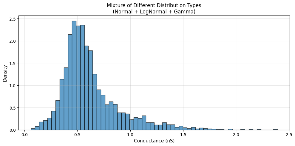
../_images/562dc03b356bbdeececa85d4a4cab7dfd32e02034cf025bf00892657ed859b16.png

💡 Mixing distribution types creates rich heterogeneity!
  Skewness: 1.61
  This matches biological observations of synaptic variability

3. Conditional Initialization#

Conditional initialization uses different distributions based on neuron properties or indices.

Use Cases#

Excitatory vs inhibitory neurons
Layer-specific properties
Cell type-specific parameters
Spatial region-specific initialization

# Example 1: Excitatory vs Inhibitory neurons
def is_excitatory(indices):
    """First 80% are excitatory, last 20% inhibitory."""
    return indices < 800

conditional_ei = init.Conditional(
    condition_fn=is_excitatory,
    true_dist=init.TruncatedNormal(
        mean=0.8 * u.nS,
        std=0.2 * u.nS,
        low=0.2 * u.nS,
        high=2.0 * u.nS
    ),  # Excitatory: positive, moderate strength
    false_dist=init.TruncatedNormal(
        mean=2.5 * u.nS,
        std=0.5 * u.nS,
        low=1.0 * u.nS,
        high=5.0 * u.nS
    )  # Inhibitory: stronger (to balance E)
)

# Generate weights
n_neurons = 1000
neuron_indices = np.arange(n_neurons)
weights_ei = conditional_ei(n_neurons, neuron_indices=neuron_indices, rng=rng)

# Separate E and I
exc_mask = is_excitatory(neuron_indices)
inh_mask = ~exc_mask

# Visualize
fig, axes = plt.subplots(1, 3, figsize=(16, 5))

# Combined histogram
axes[0].hist(weights_ei[exc_mask].mantissa, bins=40, alpha=0.6, 
             edgecolor='black', label='Excitatory (n=800)', color='red')
axes[0].hist(weights_ei[inh_mask].mantissa, bins=40, alpha=0.6, 
             edgecolor='black', label='Inhibitory (n=200)', color='blue')
axes[0].set_xlabel(f'Conductance ({weights_ei.unit})', fontsize=11)
axes[0].set_ylabel('Count', fontsize=11)
axes[0].set_title('E/I Distribution', fontsize=12)
axes[0].legend()
axes[0].grid(alpha=0.3)

# Scatter plot
colors = ['red' if e else 'blue' for e in exc_mask]
axes[1].scatter(neuron_indices, weights_ei.mantissa, c=colors, s=20, alpha=0.5)
axes[1].axhline(weights_ei[exc_mask].mean().mantissa, color='red', 
                linestyle='--', label=f'E mean: {weights_ei[exc_mask].mean():.2f}')
axes[1].axhline(weights_ei[inh_mask].mean().mantissa, color='blue', 
                linestyle='--', label=f'I mean: {weights_ei[inh_mask].mean():.2f}')
axes[1].set_xlabel('Neuron index', fontsize=11)
axes[1].set_ylabel(f'Conductance ({weights_ei.unit})', fontsize=11)
axes[1].set_title('Weight by Neuron Type', fontsize=12)
axes[1].legend()
axes[1].grid(alpha=0.3)

# Box plot comparison
axes[2].boxplot([weights_ei[exc_mask].mantissa, weights_ei[inh_mask].mantissa],
                tick_labels=['Excitatory', 'Inhibitory'],
                patch_artist=True,
                boxprops=dict(facecolor='lightgray', alpha=0.7))
axes[2].set_ylabel(f'Conductance ({weights_ei.unit})', fontsize=11)
axes[2].set_title('E/I Comparison', fontsize=12)
axes[2].grid(alpha=0.3, axis='y')

plt.tight_layout()
plt.show()

print(f"\nExcitatory neurons (n={np.sum(exc_mask)}):")
print(f"  Mean: {weights_ei[exc_mask].mean():.3f}")
print(f"  Std: {weights_ei[exc_mask].std():.3f}")
print(f"\nInhibitory neurons (n={np.sum(inh_mask)}):")
print(f"  Mean: {weights_ei[inh_mask].mean():.3f}")
print(f"  Std: {weights_ei[inh_mask].std():.3f}")
print(f"\n💡 Inhibitory synapses are ~{weights_ei[inh_mask].mean() / weights_ei[exc_mask].mean():.1f}× stronger (E/I balance)")

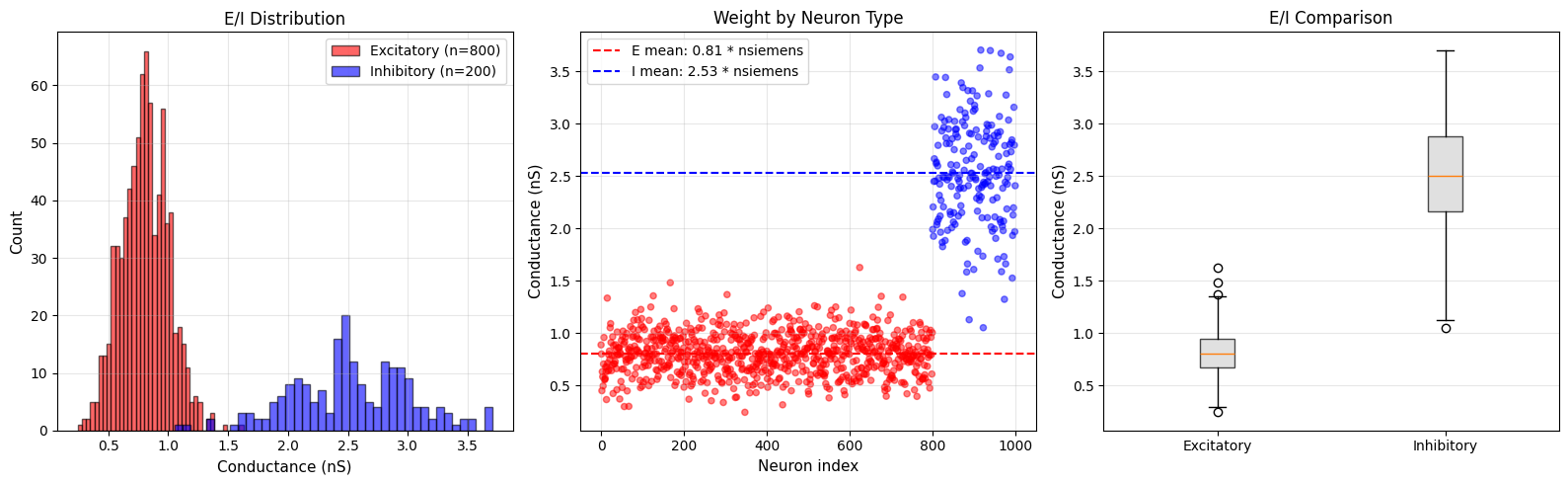
../_images/42128fbf4aedc6584bbdfde11dff22903f71d34cb8e9369d801d32a2b0191b8e.png

Excitatory neurons (n=800):
  Mean: 0.806 * nsiemens
  Std: 0.197 * nsiemens

Inhibitory neurons (n=200):
  Mean: 2.527 * nsiemens
  Std: 0.497 * nsiemens

💡 Inhibitory synapses are ~3.1× stronger (E/I balance)

Complex Conditional Logic#

# Example 2: Layer-specific initialization
def get_layer(indices):
    """
    Classify neurons into layers based on index.
    Layer 2/3: 0-400
    Layer 4: 400-600
    Layer 5: 600-1000
    """
    if hasattr(indices, '__len__'):
        layers = np.zeros_like(indices)
        layers[indices < 400] = 0  # Layer 2/3
        layers[(indices >= 400) & (indices < 600)] = 1  # Layer 4
        layers[indices >= 600] = 2  # Layer 5
        return layers
    else:
        if indices < 400:
            return 0
        elif indices < 600:
            return 1
        else:
            return 2

# Create layer-specific distributions
n_neurons = 1000
neuron_indices = np.arange(n_neurons)
layers = get_layer(neuron_indices)

# Initialize each layer separately
weights_layers = np.zeros(n_neurons)

# Layer 2/3: moderate, variable
layer23_mask = layers == 0
weights_layers[layer23_mask] = init.Normal(0.6 * u.nS, 0.15 * u.nS)(
    np.sum(layer23_mask), rng=rng
).mantissa

# Layer 4: dense, uniform
layer4_mask = layers == 1
weights_layers[layer4_mask] = init.TruncatedNormal(
    0.8 * u.nS, 0.1 * u.nS, 0.5 * u.nS, 1.2 * u.nS
)(np.sum(layer4_mask), rng=rng).mantissa

# Layer 5: strong, long-range
layer5_mask = layers == 2
weights_layers[layer5_mask] = init.LogNormal(1.2 * u.nS, 0.4 * u.nS)(
    np.sum(layer5_mask), rng=rng
).mantissa

weights_layers = weights_layers * u.nS

# Visualize
fig, axes = plt.subplots(2, 2, figsize=(14, 10))

# Histogram by layer
axes[0, 0].hist(weights_layers[layer23_mask].mantissa, bins=30, alpha=0.6, 
                label='Layer 2/3', edgecolor='black')
axes[0, 0].hist(weights_layers[layer4_mask].mantissa, bins=30, alpha=0.6, 
                label='Layer 4', edgecolor='black')
axes[0, 0].hist(weights_layers[layer5_mask].mantissa, bins=30, alpha=0.6, 
                label='Layer 5', edgecolor='black')
axes[0, 0].set_xlabel(f'Conductance ({weights_layers.unit})')
axes[0, 0].set_ylabel('Count')
axes[0, 0].set_title('Layer-Specific Distributions')
axes[0, 0].legend()
axes[0, 0].grid(alpha=0.3)

# Scatter by neuron index
layer_colors = ['blue', 'green', 'red']
colors = [layer_colors[int(l)] for l in layers]
axes[0, 1].scatter(neuron_indices, weights_layers.mantissa, c=colors, s=15, alpha=0.6)
axes[0, 1].axvline(400, color='black', linestyle='--', alpha=0.5)
axes[0, 1].axvline(600, color='black', linestyle='--', alpha=0.5)
axes[0, 1].set_xlabel('Neuron index')
axes[0, 1].set_ylabel(f'Conductance ({weights_layers.unit})')
axes[0, 1].set_title('Weight by Layer')
axes[0, 1].grid(alpha=0.3)

# Box plot
axes[1, 0].boxplot(
    [weights_layers[layer23_mask].mantissa, 
     weights_layers[layer4_mask].mantissa,
     weights_layers[layer5_mask].mantissa],
    tick_labels=['Layer 2/3', 'Layer 4', 'Layer 5'],
    patch_artist=True,
    boxprops=dict(facecolor='lightblue', alpha=0.7)
)
axes[1, 0].set_ylabel(f'Conductance ({weights_layers.unit})')
axes[1, 0].set_title('Layer Statistics')
axes[1, 0].grid(alpha=0.3, axis='y')

# Statistics table
axes[1, 1].axis('off')
stats_data = [
    ['Layer', 'N', 'Mean (nS)', 'Std (nS)', 'Range (nS)'],
    ['2/3', f'{np.sum(layer23_mask)}', 
     f'{weights_layers[layer23_mask].mean():.2f}',
     f'{weights_layers[layer23_mask].std():.2f}',
     f'[{weights_layers[layer23_mask].min():.2f}, {weights_layers[layer23_mask].max():.2f}]'],
    ['4', f'{np.sum(layer4_mask)}', 
     f'{weights_layers[layer4_mask].mean():.2f}',
     f'{weights_layers[layer4_mask].std():.2f}',
     f'[{weights_layers[layer4_mask].min():.2f}, {weights_layers[layer4_mask].max():.2f}]'],
    ['5', f'{np.sum(layer5_mask)}', 
     f'{weights_layers[layer5_mask].mean():.2f}',
     f'{weights_layers[layer5_mask].std():.2f}',
     f'[{weights_layers[layer5_mask].min():.2f}, {weights_layers[layer5_mask].max():.2f}]'],
]

table = axes[1, 1].table(cellText=stats_data, cellLoc='center', loc='center',
                         colWidths=[0.1, 0.1, 0.2, 0.2, 0.4])
table.auto_set_font_size(False)
table.set_fontsize(10)
table.scale(1, 2)
axes[1, 1].set_title('Layer Statistics Summary')

plt.tight_layout()
plt.show()

print("\n🧠 Layer-specific properties captured!")

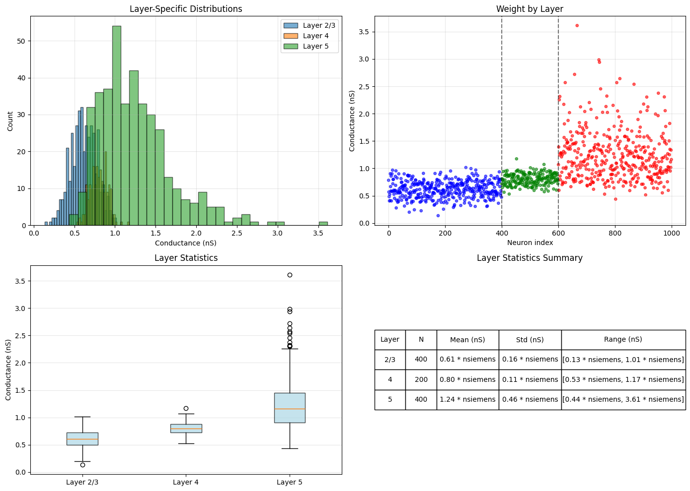
../_images/8d7efc5cd89f68fc38846bdaadfd842c9cdbd4945de549588ac4106cc8538d94.png

🧠 Layer-specific properties captured!

4. Scaled and Clipped Distributions#

Scaled Distribution#

Scaled multiplies a base distribution by a constant:

\[W_{scaled} = \alpha \cdot W_{base}\]

# Scaled distribution
base_dist = init.Normal(mean=1.0 * u.nS, std=0.2 * u.nS)

scaled_05 = init.Scaled(base_dist, scale_factor=0.5)
scaled_15 = init.Scaled(base_dist, scale_factor=1.5)
scaled_2 = init.Scaled(base_dist, scale_factor=2.0)

# Generate weights
weights_base = base_dist(1000, rng=rng)
weights_05 = scaled_05(1000, rng=rng)
weights_15 = scaled_15(1000, rng=rng)
weights_2 = scaled_2(1000, rng=rng)

# Visualize
fig, axes = plt.subplots(1, 2, figsize=(14, 5))

# Overlaid histograms
axes[0].hist(weights_base.mantissa, bins=40, alpha=0.4, label='Base (×1.0)', 
             edgecolor='black', density=True)
axes[0].hist(weights_05.mantissa, bins=40, alpha=0.4, label='Scaled (×0.5)', 
             edgecolor='black', density=True)
axes[0].hist(weights_15.mantissa, bins=40, alpha=0.4, label='Scaled (×1.5)', 
             edgecolor='black', density=True)
axes[0].hist(weights_2.mantissa, bins=40, alpha=0.4, label='Scaled (×2.0)', 
             edgecolor='black', density=True)
axes[0].set_xlabel(f'Conductance ({weights_base.unit})', fontsize=11)
axes[0].set_ylabel('Density', fontsize=11)
axes[0].set_title('Scaled Distributions', fontsize=12)
axes[0].legend()
axes[0].grid(alpha=0.3)

# Mean and std comparison
scale_factors = [0.5, 1.0, 1.5, 2.0]
means = [weights_05.mean().mantissa, weights_base.mean().mantissa, 
         weights_15.mean().mantissa, weights_2.mean().mantissa]
stds = [weights_05.std().mantissa, weights_base.std().mantissa, 
        weights_15.std().mantissa, weights_2.std().mantissa]

axes[1].plot(scale_factors, means, 'o-', linewidth=2, markersize=8, label='Mean')
axes[1].plot(scale_factors, stds, 's-', linewidth=2, markersize=8, label='Std')
axes[1].set_xlabel('Scale factor', fontsize=11)
axes[1].set_ylabel(f'Value ({weights_base.unit})', fontsize=11)
axes[1].set_title('Mean and Std vs Scale Factor', fontsize=12)
axes[1].legend()
axes[1].grid(alpha=0.3)

plt.tight_layout()
plt.show()

print("\n📏 Scaling properties:")
print(f"  Mean scales linearly with factor")
print(f"  Std also scales linearly")
print(f"  Shape (CV) remains constant")

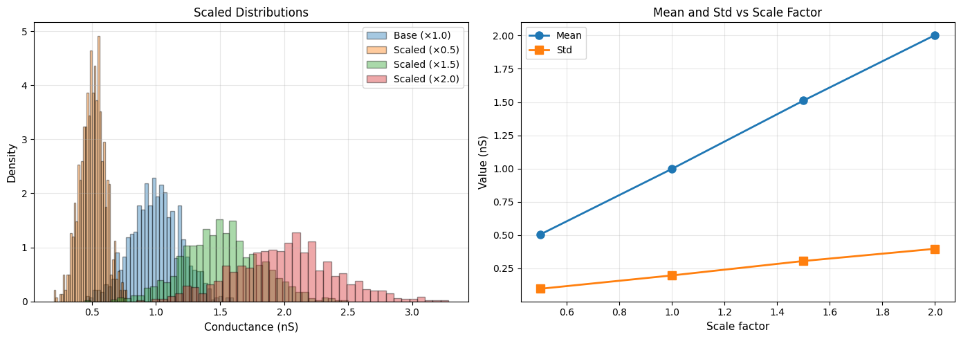
../_images/5b847cadb4301b4d1534826de8d7ee2447b06376ec7bba709cf65ef172987a6f.png

📏 Scaling properties:
  Mean scales linearly with factor
  Std also scales linearly
  Shape (CV) remains constant

Clipped Distribution#

Clipped bounds values to [min, max]:

\[W_{clipped} = \text{clip}(W_{base}, w_{min}, w_{max})\]

# Clipped distribution
base_dist = init.Normal(mean=0.5 * u.nS, std=0.3 * u.nS)

clipped_min = init.Clipped(base_dist, min_val=0.2 * u.nS, max_val=None)
clipped_max = init.Clipped(base_dist, min_val=None, max_val=0.8 * u.nS)
clipped_both = init.Clipped(base_dist, min_val=0.2 * u.nS, max_val=0.8 * u.nS)

# Generate weights
n_samples = 2000
weights_base = base_dist(n_samples, rng=rng)
weights_min = clipped_min(n_samples, rng=rng)
weights_max = clipped_max(n_samples, rng=rng)
weights_both = clipped_both(n_samples, rng=rng)

# Visualize
fig, axes = plt.subplots(2, 2, figsize=(14, 10))
axes = axes.flatten()

# Base
axes[0].hist(weights_base.mantissa, bins=50, alpha=0.7, edgecolor='black')
axes[0].set_xlabel(f'Conductance ({weights_base.unit})')
axes[0].set_ylabel('Count')
axes[0].set_title(f'Base: Normal(μ=0.5, σ=0.3)\nMean={weights_base.mean():.3f}, Std={weights_base.std():.3f}')
axes[0].grid(alpha=0.3)

# Min clipped
axes[1].hist(weights_min.mantissa, bins=50, alpha=0.7, edgecolor='black')
axes[1].axvline(0.2, color='red', linestyle='--', linewidth=2, label='Min = 0.2')
axes[1].set_xlabel(f'Conductance ({weights_min.unit})')
axes[1].set_ylabel('Count')
axes[1].set_title(f'Min Clipped\nMean={weights_min.mean():.3f}, Std={weights_min.std():.3f}')
axes[1].legend()
axes[1].grid(alpha=0.3)

# Max clipped
axes[2].hist(weights_max.mantissa, bins=50, alpha=0.7, edgecolor='black')
axes[2].axvline(0.8, color='red', linestyle='--', linewidth=2, label='Max = 0.8')
axes[2].set_xlabel(f'Conductance ({weights_max.unit})')
axes[2].set_ylabel('Count')
axes[2].set_title(f'Max Clipped\nMean={weights_max.mean():.3f}, Std={weights_max.std():.3f}')
axes[2].legend()
axes[2].grid(alpha=0.3)

# Both clipped
axes[3].hist(weights_both.mantissa, bins=50, alpha=0.7, edgecolor='black')
axes[3].axvline(0.2, color='red', linestyle='--', linewidth=2, alpha=0.7)
axes[3].axvline(0.8, color='red', linestyle='--', linewidth=2, alpha=0.7, label='Bounds')
axes[3].set_xlabel(f'Conductance ({weights_both.unit})')
axes[3].set_ylabel('Count')
axes[3].set_title(f'Both Clipped [0.2, 0.8]\nMean={weights_both.mean():.3f}, Std={weights_both.std():.3f}')
axes[3].legend()
axes[3].grid(alpha=0.3)

plt.tight_layout()
plt.show()

print("\n✂️ Clipping effects:")
print(f"  Base: {np.sum(weights_base.mantissa < 0.2)} values < 0.2, "
      f"{np.sum(weights_base.mantissa > 0.8)} values > 0.8")
print(f"  Both clipped: All values in [0.2, 0.8]")
print(f"  Clipping reduces variance: {weights_base.std():.3f} → {weights_both.std():.3f}")

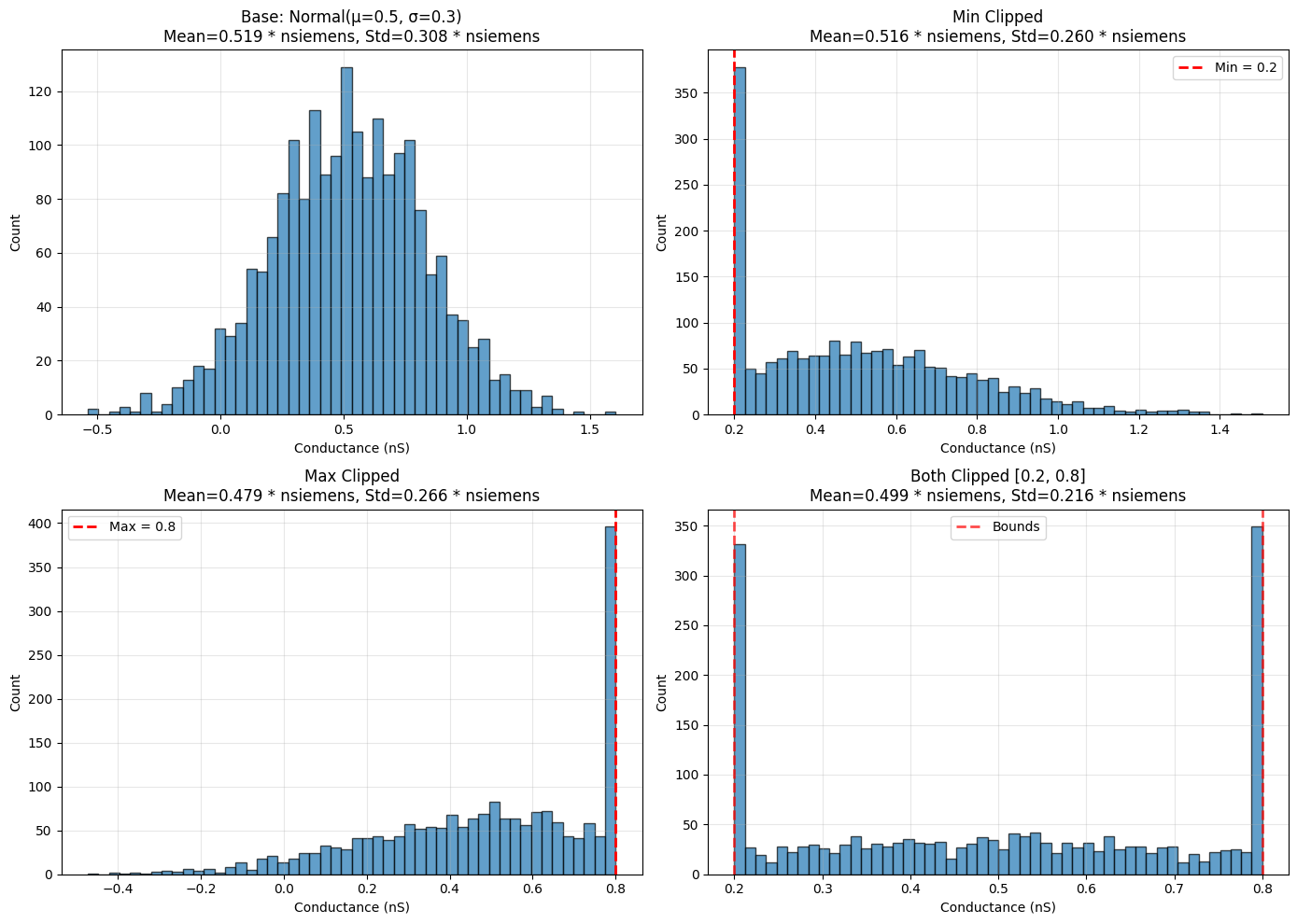
../_images/1ab147b0d9832c05bf1e056ebc737225ebd6929007588173fcb1ab776674d91c.png

✂️ Clipping effects:
  Base: 298 values < 0.2, 355 values > 0.8
  Both clipped: All values in [0.2, 0.8]
  Clipping reduces variance: 0.308 * nsiemens → 0.216 * nsiemens

5. Distance-Modulated Initialization#

DistanceModulated combines a base weight distribution with a distance-dependent profile:

\[W(d) = W_{base} \cdot f(d)\]

where:

\(W_{base}\): Base weight distribution
\(f(d)\): Distance profile
\(d\): Spatial distance between neurons

This creates spatially structured connectivity patterns.

# Example 1: Gaussian distance modulation
base_weights = init.Normal(mean=1.0 * u.nS, std=0.2 * u.nS)
gaussian_profile = init.GaussianProfile(sigma=100.0 * u.um)

distance_modulated = init.DistanceModulated(
    base_dist=base_weights,
    distance_profile=gaussian_profile,
    min_weight=0.05 * u.nS  # Floor to ensure some connectivity
)

# Create distance array
n_connections = 1000
distances = np.random.uniform(0, 300, n_connections) * u.um

# Generate modulated weights
weights_modulated = distance_modulated(n_connections, distances=distances, rng=rng)
weights_unmodulated = base_weights(n_connections, rng=rng)

# Visualize
fig, axes = plt.subplots(2, 2, figsize=(14, 10))

# Distance profile
dist_range = np.linspace(0, 300, 500) * u.um
profile_values = gaussian_profile.probability(dist_range)
axes[0, 0].plot(dist_range.mantissa, profile_values, linewidth=2)
axes[0, 0].fill_between(dist_range.mantissa, profile_values, alpha=0.3)
axes[0, 0].set_xlabel('Distance (μm)')
axes[0, 0].set_ylabel('Modulation factor')
axes[0, 0].set_title('Gaussian Distance Profile (σ=100 μm)')
axes[0, 0].grid(alpha=0.3)

# Unmodulated weights
axes[0, 1].hist(weights_unmodulated.mantissa, bins=50, alpha=0.7, edgecolor='black')
axes[0, 1].set_xlabel(f'Conductance ({weights_unmodulated.unit})')
axes[0, 1].set_ylabel('Count')
axes[0, 1].set_title(f'Unmodulated Weights\nMean={weights_unmodulated.mean():.3f}')
axes[0, 1].grid(alpha=0.3)

# Modulated weights histogram
axes[1, 0].hist(weights_modulated.mantissa, bins=50, alpha=0.7, 
                edgecolor='black', color='orange')
axes[1, 0].axvline(0.05, color='red', linestyle='--', label='Min weight')
axes[1, 0].set_xlabel(f'Conductance ({weights_modulated.unit})')
axes[1, 0].set_ylabel('Count')
axes[1, 0].set_title(f'Distance-Modulated Weights\nMean={weights_modulated.mean():.3f}')
axes[1, 0].legend()
axes[1, 0].grid(alpha=0.3)

# Scatter: weight vs distance
scatter = axes[1, 1].scatter(distances.mantissa, weights_modulated.mantissa, 
                             c=weights_modulated.mantissa, cmap='viridis', 
                             s=30, alpha=0.6)
axes[1, 1].set_xlabel('Distance (μm)')
axes[1, 1].set_ylabel(f'Conductance ({weights_modulated.unit})')
axes[1, 1].set_title('Weight vs Distance')
plt.colorbar(scatter, ax=axes[1, 1], label='Conductance (nS)')
axes[1, 1].grid(alpha=0.3)

plt.tight_layout()
plt.show()

print(f"\n🌍 Distance modulation effects:")
print(f"  Unmodulated mean: {weights_unmodulated.mean():.3f}")
print(f"  Modulated mean: {weights_modulated.mean():.3f}")
print(f"  Close connections (< 50 μm) mean: {weights_modulated[distances.mantissa < 50].mean():.3f}")
print(f"  Far connections (> 200 μm) mean: {weights_modulated[distances.mantissa > 200].mean():.3f}")

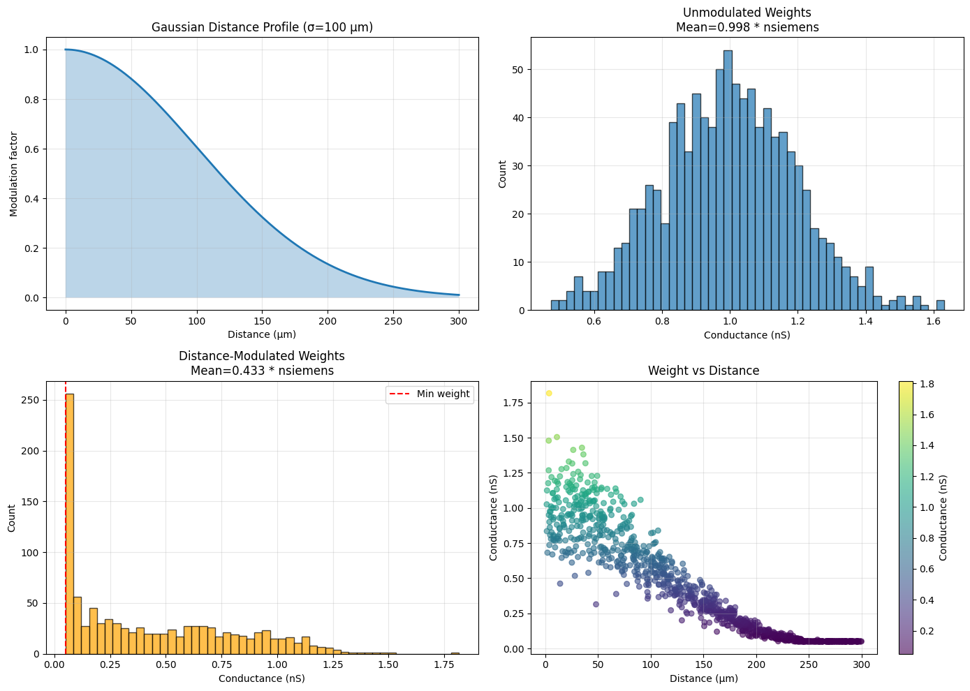
../_images/78e8cdded6e5623ab3035692d54b7540476fd227c7d3f6cd14cbf9bfecd37b7a.png

🌍 Distance modulation effects:
  Unmodulated mean: 0.998 * nsiemens
  Modulated mean: 0.433 * nsiemens
  Close connections (< 50 μm) mean: 0.966 * nsiemens
  Far connections (> 200 μm) mean: 0.065 * nsiemens

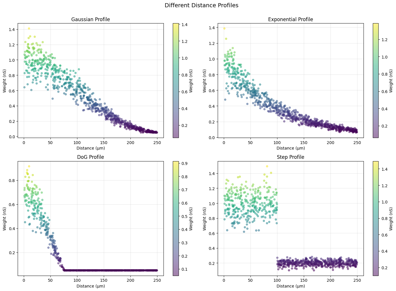
Different Distance Profiles#

# Compare different distance profiles
base = init.Normal(1.0 * u.nS, 0.15 * u.nS)

profiles = {
    'Gaussian': init.GaussianProfile(sigma=100.0 * u.um),
    'Exponential': init.ExponentialProfile(decay_constant=100.0 * u.um),
    'DoG': init.DoGProfile(sigma_center=50.0 * u.um, sigma_surround=150.0 * u.um,
                           amplitude_center=1.0, amplitude_surround=0.3),
    'Step': init.StepProfile(threshold=100.0 * u.um, inside_prob=1.0, outside_prob=0.2),
}

# Generate distances
n_samples = 800
distances = np.random.uniform(0, 250, n_samples) * u.um

# Visualize
fig, axes = plt.subplots(2, 2, figsize=(14, 10))
axes = axes.flatten()

for ax, (name, profile) in zip(axes, profiles.items()):
    # Create distance-modulated initializer
    dm = init.DistanceModulated(base, profile, min_weight=0.05 * u.nS)
    weights = dm(n_samples, distances=distances, rng=rng)
    
    # Scatter plot
    scatter = ax.scatter(distances.mantissa, weights.mantissa, 
                        c=weights.mantissa, cmap='viridis', s=20, alpha=0.5)
    ax.set_xlabel('Distance (μm)')
    ax.set_ylabel(f'Weight ({weights.unit})')
    ax.set_title(f'{name} Profile')
    ax.grid(alpha=0.3)
    plt.colorbar(scatter, ax=ax, label='Weight (nS)')

plt.suptitle('Different Distance Profiles', fontsize=14, y=1.00)
plt.tight_layout()
plt.show()

print("\n📊 Profile comparison:")
print("  Gaussian: Smooth decay, strongest at center")
print("  Exponential: Monotonic decay with heavier tail")
print("  DoG: Center-surround with lateral inhibition")
print("  Step: Binary connectivity regions")

../_images/d2bf83908dd86311086ef404f3adcabacb1d44cd043f9ff0c3f9dd6d07b6b1d1.png

📊 Profile comparison:
  Gaussian: Smooth decay, strongest at center
  Exponential: Monotonic decay with heavier tail
  DoG: Center-surround with lateral inhibition
  Step: Binary connectivity regions

6. Building Complex Initialization Schemes#

Now let’s combine multiple techniques to create sophisticated initialization patterns.

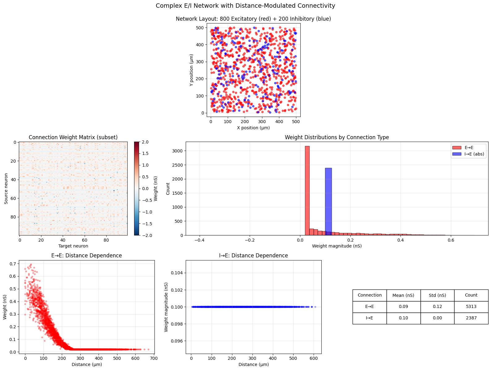
Scheme 1: E/I Network with Distance Modulation#

# Create E/I network with distance-dependent connectivity
n_exc = 800
n_inh = 200
n_total = n_exc + n_inh

# Generate random 2D positions
np.random.seed(42)
positions = np.random.uniform(0, 500, (n_total, 2))  # μm

# Create connectivity matrix (subset for visualization)
n_show = 100  # Show subset
source_idx = np.random.choice(n_total, n_show, replace=False)
target_idx = np.random.choice(n_total, n_show, replace=False)

# Compute distances
distances = np.linalg.norm(
    positions[source_idx][:, np.newaxis, :] - positions[target_idx][np.newaxis, :, :],
    axis=2
) * u.um

# Initialize E→E connections
exc_profile = init.GaussianProfile(sigma=100.0 * u.um)
exc_base = init.Normal(0.5 * u.nS, 0.1 * u.nS)
exc_init = init.DistanceModulated(exc_base, exc_profile, min_weight=0.02 * u.nS)

# Initialize E→I connections
ei_profile = init.ExponentialProfile(decay_constant=150.0 * u.um)
ei_base = init.Normal(0.6 * u.nS, 0.12 * u.nS)
ei_init = init.DistanceModulated(ei_base, ei_profile, min_weight=0.05 * u.nS)

# Initialize I→E connections (lateral inhibition)
ie_profile = init.DoGProfile(
    sigma_center=60.0 * u.um, sigma_surround=180.0 * u.um,
    amplitude_center=0.5, amplitude_surround=0.6
).clip(min_val=0.0, max_val=1.0)
ie_base = init.LogNormal(1.5 * u.nS, 0.4 * u.nS)
ie_init = init.DistanceModulated(ie_base, ie_profile, min_weight=0.1 * u.nS)

# Initialize I→I connections
ii_profile = init.GaussianProfile(sigma=80.0 * u.um)
ii_base = init.Normal(0.8 * u.nS, 0.15 * u.nS)
ii_init = init.DistanceModulated(ii_base, ii_profile, min_weight=0.05 * u.nS)

# Generate connection weights
weights_matrix = np.zeros((n_show, n_show))

for i, src in enumerate(source_idx):
    for j, tgt in enumerate(target_idx):
        dist = distances[i, j:j+1]
        
        if src < n_exc and tgt < n_exc:  # E→E
            weights_matrix[i, j] = exc_init(1, distances=dist, rng=rng).mantissa[0]
        elif src < n_exc and tgt >= n_exc:  # E→I
            weights_matrix[i, j] = ei_init(1, distances=dist, rng=rng).mantissa[0]
        elif src >= n_exc and tgt < n_exc:  # I→E
            weights_matrix[i, j] = -ie_init(1, distances=dist, rng=rng).mantissa[0]  # Negative for inhibition
        else:  # I→I
            weights_matrix[i, j] = -ii_init(1, distances=dist, rng=rng).mantissa[0]

# Visualize
fig = plt.figure(figsize=(16, 12))
gs = GridSpec(3, 3, figure=fig)

# Network layout
ax1 = fig.add_subplot(gs[0, :])
colors = ['red'] * n_exc + ['blue'] * n_inh
ax1.scatter(positions[:, 0], positions[:, 1], c=colors, s=20, alpha=0.6)
ax1.set_xlabel('X position (μm)')
ax1.set_ylabel('Y position (μm)')
ax1.set_title(f'Network Layout: {n_exc} Excitatory (red) + {n_inh} Inhibitory (blue)')
ax1.set_aspect('equal')
ax1.grid(alpha=0.3)

# Connection matrix
ax2 = fig.add_subplot(gs[1, 0])
im = ax2.imshow(weights_matrix, cmap='RdBu_r', vmin=-2, vmax=2, aspect='auto')
ax2.set_xlabel('Target neuron')
ax2.set_ylabel('Source neuron')
ax2.set_title('Connection Weight Matrix (subset)')
plt.colorbar(im, ax=ax2, label='Weight (nS)')

# Weight distribution by type
ax3 = fig.add_subplot(gs[1, 1:])
exc_weights = weights_matrix[source_idx < n_exc][:, target_idx < n_exc].flatten()
exc_weights = exc_weights[exc_weights != 0]
inh_weights = weights_matrix[source_idx >= n_exc][:, target_idx < n_exc].flatten()
inh_weights = inh_weights[inh_weights != 0]

ax3.hist(exc_weights, bins=40, alpha=0.6, label='E→E', color='red', edgecolor='black')
ax3.hist(np.abs(inh_weights), bins=40, alpha=0.6, label='I→E (abs)', color='blue', edgecolor='black')
ax3.set_xlabel('Weight magnitude (nS)')
ax3.set_ylabel('Count')
ax3.set_title('Weight Distributions by Connection Type')
ax3.legend()
ax3.grid(alpha=0.3)

# Distance dependence
ax4 = fig.add_subplot(gs[2, 0])
exc_dists = distances.mantissa[source_idx < n_exc][:, target_idx < n_exc].flatten()
exc_w = weights_matrix[source_idx < n_exc][:, target_idx < n_exc].flatten()
mask = exc_w != 0
ax4.scatter(exc_dists[mask], exc_w[mask], alpha=0.3, s=10, color='red')
ax4.set_xlabel('Distance (μm)')
ax4.set_ylabel('Weight (nS)')
ax4.set_title('E→E: Distance Dependence')
ax4.grid(alpha=0.3)

# I→E distance dependence
ax5 = fig.add_subplot(gs[2, 1])
inh_dists = distances.mantissa[source_idx >= n_exc][:, target_idx < n_exc].flatten()
inh_w = weights_matrix[source_idx >= n_exc][:, target_idx < n_exc].flatten()
mask = inh_w != 0
ax5.scatter(inh_dists[mask], np.abs(inh_w[mask]), alpha=0.3, s=10, color='blue')
ax5.set_xlabel('Distance (μm)')
ax5.set_ylabel('Weight magnitude (nS)')
ax5.set_title('I→E: Distance Dependence')
ax5.grid(alpha=0.3)

# Statistics table
ax6 = fig.add_subplot(gs[2, 2])
ax6.axis('off')
stats = [
    ['Connection', 'Mean (nS)', 'Std (nS)', 'Count'],
    ['E→E', f'{np.mean(exc_weights):.2f}', f'{np.std(exc_weights):.2f}', f'{len(exc_weights)}'],
    ['I→E', f'{np.mean(np.abs(inh_weights)):.2f}', f'{np.std(np.abs(inh_weights)):.2f}', f'{len(inh_weights)}'],
]
table = ax6.table(cellText=stats, cellLoc='center', loc='center')
table.auto_set_font_size(False)
table.set_fontsize(10)
table.scale(1, 2)

plt.suptitle('Complex E/I Network with Distance-Modulated Connectivity', fontsize=14, y=0.995)
plt.tight_layout()
plt.show()

print("\n🧠 E/I Network created with:")
print("  ✓ Distance-dependent E→E (Gaussian)")
print("  ✓ Distance-dependent E→I (Exponential)")
print("  ✓ Lateral inhibition I→E (DoG)")
print("  ✓ Local I→I (Gaussian)")

../_images/40a6604eb13dba612075353dfb57e9a3464009788cb67c551561914a138253cf.png

🧠 E/I Network created with:
  ✓ Distance-dependent E→E (Gaussian)
  ✓ Distance-dependent E→I (Exponential)
  ✓ Lateral inhibition I→E (DoG)
  ✓ Local I→I (Gaussian)

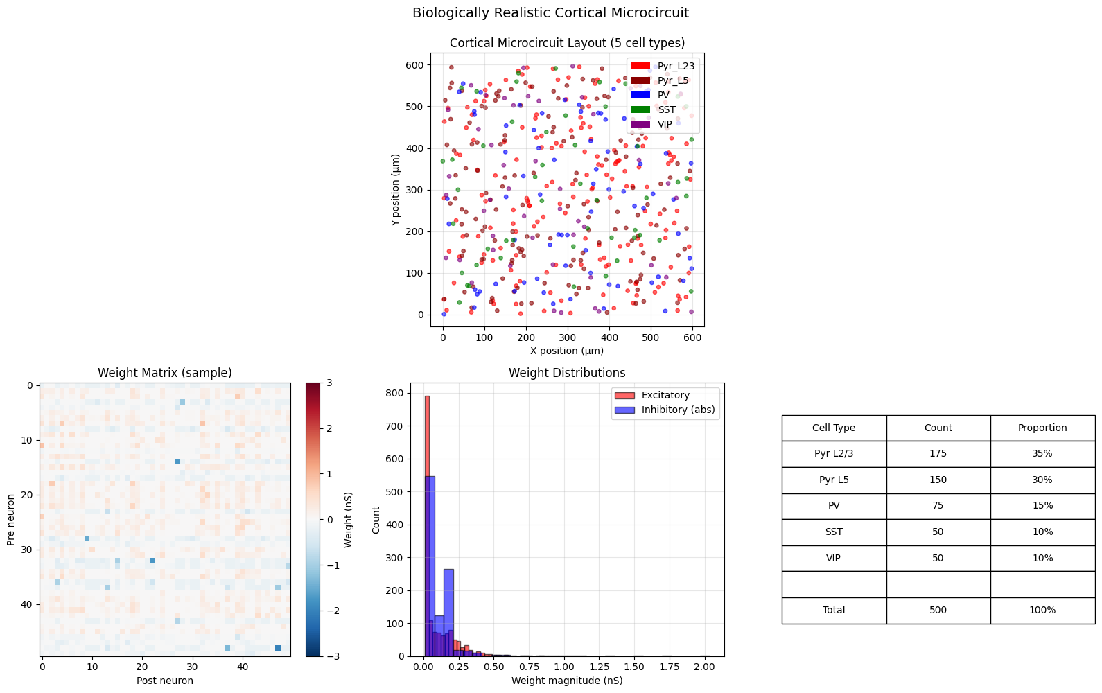
7. Integration Example: Biologically Realistic Cortical Circuit#

Let’s create a complete cortical microcircuit with:

Multiple cell types
Layer-specific connectivity
Distance-dependent patterns
Heterogeneous weights

# Define cortical microcircuit
class CorticalMicrocircuit:
    def __init__(self, n_neurons=500, spatial_extent=600.0):
        self.n_neurons = n_neurons
        self.spatial_extent = spatial_extent  # μm
        
        # Cell type proportions (simplified)
        self.n_pyr_l23 = int(0.35 * n_neurons)  # Pyramidal L2/3
        self.n_pyr_l5 = int(0.30 * n_neurons)   # Pyramidal L5
        self.n_pv = int(0.15 * n_neurons)       # Parvalbumin interneurons
        self.n_sst = int(0.10 * n_neurons)      # Somatostatin interneurons
        self.n_vip = int(0.10 * n_neurons)      # VIP interneurons
        
        # Generate positions
        self.positions = np.random.uniform(0, spatial_extent, (n_neurons, 2))
        
        # Cell type labels
        self.cell_types = (
            ['Pyr_L23'] * self.n_pyr_l23 +
            ['Pyr_L5'] * self.n_pyr_l5 +
            ['PV'] * self.n_pv +
            ['SST'] * self.n_sst +
            ['VIP'] * self.n_vip
        )
        
    def get_connection_params(self, pre_type, post_type):
        """Get initialization parameters for specific connection type."""
        
        params = {
            # Excitatory connections
            ('Pyr_L23', 'Pyr_L23'): {
                'base': init.Normal(0.4 * u.nS, 0.08 * u.nS),
                'profile': init.GaussianProfile(sigma=120.0 * u.um),
                'min_weight': 0.02 * u.nS
            },
            ('Pyr_L23', 'Pyr_L5'): {
                'base': init.Normal(0.6 * u.nS, 0.12 * u.nS),
                'profile': init.ExponentialProfile(decay_constant=150.0 * u.um),
                'min_weight': 0.03 * u.nS
            },
            ('Pyr_L5', 'Pyr_L5'): {
                'base': init.LogNormal(0.8 * u.nS, 0.3 * u.nS),
                'profile': init.BimodalProfile(
                    sigma1=80.0 * u.um, sigma2=200.0 * u.um,
                    center1=0.0 * u.um, center2=300.0 * u.um,
                    amplitude1=0.8, amplitude2=0.3
                ),
                'min_weight': 0.05 * u.nS
            },
            
            # Inhibitory connections
            ('PV', 'Pyr_L23'): {
                'base': init.Normal(2.0 * u.nS, 0.4 * u.nS),
                'profile': init.GaussianProfile(sigma=60.0 * u.um),
                'min_weight': 0.2 * u.nS
            },
            ('SST', 'Pyr_L5'): {
                'base': init.Normal(1.5 * u.nS, 0.3 * u.nS),
                'profile': init.DoGProfile(
                    sigma_center=50.0 * u.um, sigma_surround=150.0 * u.um,
                    amplitude_center=0.8, amplitude_surround=0.4
                ),
                'min_weight': 0.1 * u.nS
            },
        }
        
        # Default for undefined connections
        default = {
            'base': init.Normal(0.3 * u.nS, 0.1 * u.nS),
            'profile': init.GaussianProfile(sigma=100.0 * u.um),
            'min_weight': 0.01 * u.nS
        }
        
        return params.get((pre_type, post_type), default)
    
    def initialize_connection(self, pre_idx, post_idx, rng):
        """Initialize a single connection."""
        pre_type = self.cell_types[pre_idx]
        post_type = self.cell_types[post_idx]
        
        # Compute distance
        dist = np.linalg.norm(self.positions[pre_idx] - self.positions[post_idx])
        distance = np.array([dist]) * u.um
        
        # Get parameters
        params = self.get_connection_params(pre_type, post_type)
        
        # Create distance-modulated initializer
        dm_init = init.DistanceModulated(
            base_dist=params['base'],
            distance_profile=params['profile'],
        ).clip(min_val=params['min_weight'])
        
        # Generate weight
        weight = dm_init(1, distances=distance, rng=rng).mantissa[0]
        
        # Make inhibitory connections negative
        if pre_type in ['PV', 'SST', 'VIP']:
            weight = -weight
        
        return weight

# Create microcircuit
print("Creating cortical microcircuit...")
circuit = CorticalMicrocircuit(n_neurons=500)

# Sample connections for visualization
n_sample = 50
pre_sample = np.random.choice(circuit.n_neurons, n_sample, replace=False)
post_sample = np.random.choice(circuit.n_neurons, n_sample, replace=False)

# Initialize sampled connections
rng = np.random.default_rng(42)
weights_sample = np.zeros((n_sample, n_sample))

for i, pre in enumerate(pre_sample):
    for j, post in enumerate(post_sample):
        if pre != post:  # No self-connections
            weights_sample[i, j] = circuit.initialize_connection(pre, post, rng)

print("Microcircuit initialized!")

# Visualize
fig = plt.figure(figsize=(16, 10))
gs = GridSpec(2, 3, figure=fig)

# Network layout with cell types
ax1 = fig.add_subplot(gs[0, :])
type_colors = {
    'Pyr_L23': 'red', 'Pyr_L5': 'darkred',
    'PV': 'blue', 'SST': 'green', 'VIP': 'purple'
}
colors = [type_colors[ct] for ct in circuit.cell_types]
ax1.scatter(circuit.positions[:, 0], circuit.positions[:, 1], 
           c=colors, s=15, alpha=0.6)

# Legend
from matplotlib.patches import Patch
legend_elements = [Patch(facecolor=color, label=cell_type) 
                  for cell_type, color in type_colors.items()]
ax1.legend(handles=legend_elements, loc='upper right')
ax1.set_xlabel('X position (μm)')
ax1.set_ylabel('Y position (μm)')
ax1.set_title('Cortical Microcircuit Layout (5 cell types)')
ax1.set_aspect('equal')
ax1.grid(alpha=0.3)

# Connection matrix
ax2 = fig.add_subplot(gs[1, 0])
im = ax2.imshow(weights_sample, cmap='RdBu_r', vmin=-3, vmax=3, aspect='auto')
ax2.set_xlabel('Post neuron')
ax2.set_ylabel('Pre neuron')
ax2.set_title('Weight Matrix (sample)')
plt.colorbar(im, ax=ax2, label='Weight (nS)')

# Weight distribution
ax3 = fig.add_subplot(gs[1, 1])
exc_weights = weights_sample[weights_sample > 0]
inh_weights = weights_sample[weights_sample < 0]
ax3.hist(exc_weights, bins=30, alpha=0.6, label='Excitatory', color='red', edgecolor='black')
ax3.hist(np.abs(inh_weights), bins=30, alpha=0.6, label='Inhibitory (abs)', 
        color='blue', edgecolor='black')
ax3.set_xlabel('Weight magnitude (nS)')
ax3.set_ylabel('Count')
ax3.set_title('Weight Distributions')
ax3.legend()
ax3.grid(alpha=0.3)

# Statistics
ax4 = fig.add_subplot(gs[1, 2])
ax4.axis('off')
stats = [
    ['Cell Type', 'Count', 'Proportion'],
    ['Pyr L2/3', str(circuit.n_pyr_l23), '35%'],
    ['Pyr L5', str(circuit.n_pyr_l5), '30%'],
    ['PV', str(circuit.n_pv), '15%'],
    ['SST', str(circuit.n_sst), '10%'],
    ['VIP', str(circuit.n_vip), '10%'],
    ['', '', ''],
    ['Total', str(circuit.n_neurons), '100%'],
]
table = ax4.table(cellText=stats, cellLoc='center', loc='center')
table.auto_set_font_size(False)
table.set_fontsize(10)
table.scale(1, 2)

plt.suptitle('Biologically Realistic Cortical Microcircuit', fontsize=14, y=0.995)
plt.tight_layout()
plt.show()

print(f"\n🎯 Microcircuit statistics:")
print(f"  Total neurons: {circuit.n_neurons}")
print(f"  Excitatory: {circuit.n_pyr_l23 + circuit.n_pyr_l5} ({100*(circuit.n_pyr_l23 + circuit.n_pyr_l5)/circuit.n_neurons:.0f}%)")
print(f"  Inhibitory: {circuit.n_pv + circuit.n_sst + circuit.n_vip} ({100*(circuit.n_pv + circuit.n_sst + circuit.n_vip)/circuit.n_neurons:.0f}%)")
print(f"\n  Sampled connections: {n_sample}×{n_sample} = {n_sample**2}")
print(f"  Non-zero weights: {np.sum(weights_sample != 0)}")
print(f"  Excitatory weights: mean={np.mean(exc_weights):.2f} nS, std={np.std(exc_weights):.2f} nS")
print(f"  Inhibitory weights: mean={np.mean(np.abs(inh_weights)):.2f} nS, std={np.std(np.abs(inh_weights)):.2f} nS")

Creating cortical microcircuit...
Microcircuit initialized!

../_images/8db542d3a4cb089c4c8c339fecd7cff6299d68a4ed5b3cd139d90e3bea38a697.png

🎯 Microcircuit statistics:
  Total neurons: 500
  Excitatory: 325 (65%)
  Inhibitory: 175 (35%)

  Sampled connections: 50×50 = 2500
  Non-zero weights: 2496
  Excitatory weights: mean=0.10 nS, std=0.12 nS
  Inhibitory weights: mean=0.11 nS, std=0.17 nS

Summary#

In this tutorial, we covered:

Mixture distributions: Creating heterogeneous populations
Conditional initialization: Cell type-specific properties
Scaled/Clipped distributions: Transforming base distributions
DistanceModulated: Spatially structured connectivity
Complex schemes: Combining multiple strategies
Biological realism: Complete cortical microcircuit

Design Patterns:

Pattern	Use Case	Example
Mixture	Multiple synapse types	Weak + strong synapses
Conditional	Cell type differences	E vs I neurons
Scaled	Global modulation	Activity-dependent scaling
Clipped	Biological bounds	Ensure positive conductances
DistanceModulated	Spatial structure	Local vs long-range
Combined	Realistic circuits	All of the above

Tutorial 4: Composite and Distance-Modulated Initialization Strategies

Contents

Tutorial 4: Composite and Distance-Modulated Initialization Strategies#

Topics Covered#

Installation and Setup#

1. Introduction to Composite Initialization#

Why Composite Initialization?#

Types of Composition#

Key Principles#

2. Mixture Distributions#

Mathematical Definition#

Use Cases#

Multi-Component Mixture#

Mixture with Different Distribution Types#

3. Conditional Initialization#

Use Cases#

Complex Conditional Logic#

4. Scaled and Clipped Distributions#

Scaled Distribution#

Clipped Distribution#

5. Distance-Modulated Initialization#

Different Distance Profiles#

6. Building Complex Initialization Schemes#

Scheme 1: E/I Network with Distance Modulation#

7. Integration Example: Biologically Realistic Cortical Circuit#

Summary#