
Tutorial 2: Advanced Initialization - Variance Scaling and Orthogonal Methods#
![]()
This tutorial covers advanced weight initialization strategies that are essential for training deep neural networks effectively. These methods automatically scale initialization based on network architecture to maintain stable gradient flow.
Topics Covered#
Variance scaling principles for deep networks
Kaiming/He initialization for ReLU networks
Xavier/Glorot initialization for tanh/sigmoid
LeCun initialization for SELU
Orthogonal initialization for RNNs and deep CNNs
Identity initialization
Fan modes explained: fan-in, fan-out, fan-avg
Installation and Setup#
# Install braintools if needed
# !pip install braintools brainunit matplotlib numpy jax
import numpy as np
import matplotlib.pyplot as plt
import brainunit as u
from braintools import init
import jax.numpy as jnp

# Set random seed for reproducibility
np.random.seed(42)

# Configure matplotlib
plt.rcParams['figure.figsize'] = (12, 4)
plt.rcParams['font.size'] = 10
1. Variance Scaling Principles#
The Problem: Vanishing and Exploding Gradients#
In deep networks, improper initialization can cause:
Vanishing gradients: Signals become too small as they propagate
Exploding gradients: Signals become too large as they propagate
Both problems make training difficult or impossible.
The Solution: Variance Scaling#
Variance scaling methods initialize weights based on the network’s fan-in (number of input units) and/or fan-out (number of output units) to maintain signal variance across layers.
Key principle: Initialize weights so that:
Forward pass: activations maintain similar variance
Backward pass: gradients maintain similar variance
Mathematical Foundation#
For a linear layer with input \(x\) and weights \(W\):
The variance of the output is:
To maintain \(\text{Var}(y) = \text{Var}(x)\), we need:
Visualizing the Gradient Problem#
def simulate_forward_pass(n_layers, n_units, init_std, activation='linear'):
    """
    Simulate forward pass through a deep network.
    """
    # Initialize input
    x = np.random.randn(1000, n_units)

    # Track activation statistics
    means = [x.mean()]
    stds = [x.std()]

    for layer in range(n_layers):
        # Weight matrix
        W = np.random.randn(n_units, n_units) * init_std

        # Forward pass
        x = x @ W

        # Apply activation
        if activation == 'relu':
            x = np.maximum(0, x)
        elif activation == 'tanh':
            x = np.tanh(x)

        means.append(x.mean())
        stds.append(x.std())

    return means, stds

# Compare different initialization scales
n_layers = 20
n_units = 100

# Too small initialization
means_small, stds_small = simulate_forward_pass(n_layers, n_units, 0.01)

# Too large initialization
means_large, stds_large = simulate_forward_pass(n_layers, n_units, 1.0)

# Properly scaled initialization
means_good, stds_good = simulate_forward_pass(n_layers, n_units, 1.0 / np.sqrt(n_units))

# Visualize
fig, axes = plt.subplots(1, 2, figsize=(14, 5))

# Standard deviation across layers
layers = np.arange(len(stds_small))
axes[0].semilogy(layers, stds_small, 'o-', label='Too small (std=0.01)', linewidth=2)
axes[0].semilogy(layers, stds_large, 's-', label='Too large (std=1.0)', linewidth=2)
axes[0].semilogy(layers, stds_good, '^-', label='Properly scaled (std=1/√n)', linewidth=2)
axes[0].axhline(1.0, color='red', linestyle='--', alpha=0.5, label='Target')
axes[0].set_xlabel('Layer depth')
axes[0].set_ylabel('Activation std (log scale)')
axes[0].set_title('Signal Propagation Through Deep Network')
axes[0].legend()
axes[0].grid(alpha=0.3)

# Mean across layers
axes[1].plot(layers, means_small, 'o-', label='Too small', linewidth=2)
axes[1].plot(layers, means_large, 's-', label='Too large', linewidth=2)
axes[1].plot(layers, means_good, '^-', label='Properly scaled', linewidth=2)
axes[1].axhline(0.0, color='red', linestyle='--', alpha=0.5, label='Target')
axes[1].set_xlabel('Layer depth')
axes[1].set_ylabel('Activation mean')
axes[1].set_title('Mean Activation Through Deep Network')
axes[1].legend()
axes[1].grid(alpha=0.3)

plt.tight_layout()
plt.show()

print("\n⚠️ Problems with improper initialization:")
print(f"  Too small: Final std = {stds_small[-1]:.2e} (vanishing signals)")
print(f"  Too large: Final std = {stds_large[-1]:.2e} (exploding signals)")
print(f"  Properly scaled: Final std = {stds_good[-1]:.2f} (stable signals)")
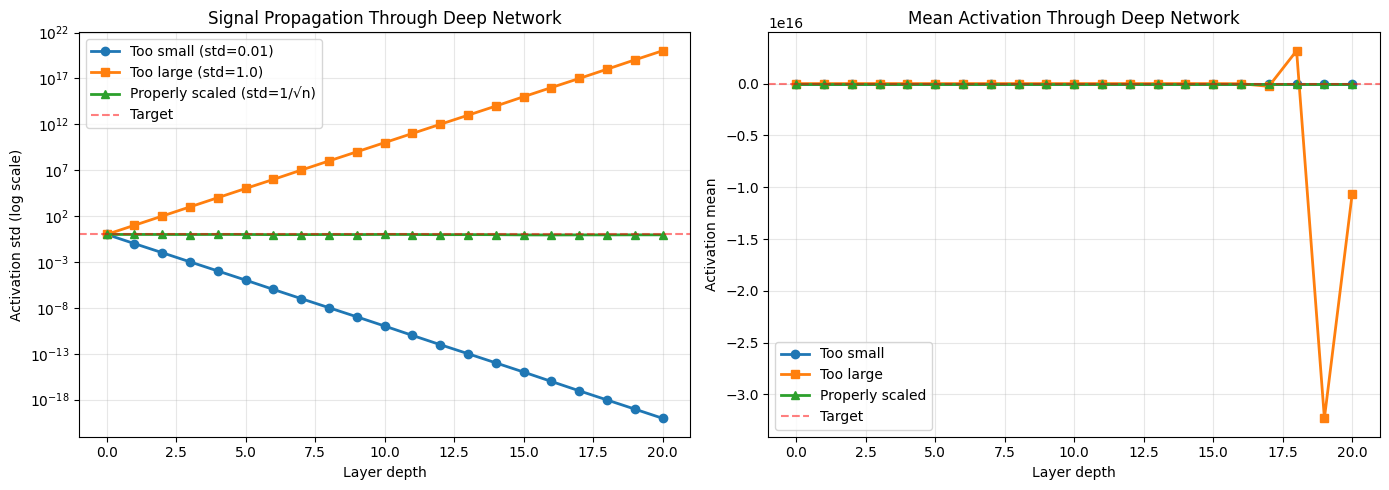
⚠️ Problems with improper initialization:
  Too small: Final std = 9.12e-21 (vanishing signals)
  Too large: Final std = 1.05e+20 (exploding signals)
  Properly scaled: Final std = 0.90 (stable signals)
2. Fan Modes Explained#
Before diving into specific methods, let’s understand the fan concept:
Fan-in and Fan-out#
For a weight matrix \(W\) of shape \((n_{out}, n_{in})\):
Fan-in (\(n_{in}\)): Number of input connections to each neuron
Fan-out (\(n_{out}\)): Number of output connections from each neuron
Fan-avg: Average of fan-in and fan-out: \((n_{in} + n_{out}) / 2\)
Which mode to use?#
fan_in: Focus on forward pass stability (Kaiming, LeCun)
fan_out: Focus on backward pass (gradient) stability
fan_avg: Balance between forward and backward (Xavier/Glorot)
For higher-dimensional tensors (e.g., convolution kernels):
Receptive field size is also considered
Example: Conv2D kernel of shape \((C_{out}, C_{in}, H, W)\)
fan_in = \(C_{in} \times H \times W\)
fan_out = \(C_{out} \times H \times W\)
# Visualize fan computation for different layer types
import pandas as pd

examples = [
    ('Dense 100→50', (50, 100), 100, 50, 75),
    ('Dense 50→100', (100, 50), 50, 100, 75),
    ('Conv2D 3×3, 16→32', (32, 16, 3, 3), 16*3*3, 32*3*3, (16*3*3 + 32*3*3)/2),
    ('Conv2D 5×5, 64→128', (128, 64, 5, 5), 64*5*5, 128*5*5, (64*5*5 + 128*5*5)/2),
]

df = pd.DataFrame(examples, columns=['Layer Type', 'Shape', 'Fan-in', 'Fan-out', 'Fan-avg'])
print("\nFan Computation Examples:")
print("=" * 80)
print(df.to_string(index=False))
print("=" * 80)

# Visualize how fan affects initialization variance
fig, ax = plt.subplots(1, 1, figsize=(10, 6))

fans = [10, 50, 100, 500, 1000]
var_fan_in = [1.0 / f for f in fans]
var_fan_out = [1.0 / f for f in fans]
var_fan_avg = [2.0 / f for f in fans]  # Xavier uses 2/fan_avg

ax.loglog(fans, var_fan_in, 'o-', label='Var(w) = 1/fan_in', linewidth=2, markersize=8)
ax.loglog(fans, var_fan_avg, 's-', label='Var(w) = 2/fan_avg', linewidth=2, markersize=8)
ax.set_xlabel('Number of connections (fan)', fontsize=12)
ax.set_ylabel('Weight variance', fontsize=12)
ax.set_title('Weight Variance vs Fan Size', fontsize=14)
ax.legend(fontsize=11)
ax.grid(alpha=0.3)

plt.tight_layout()
plt.show()

print("\n📊 Key insight: Variance decreases as fan increases to maintain signal scale")
Fan Computation Examples:
================================================================================
        Layer Type           Shape  Fan-in  Fan-out  Fan-avg
      Dense 100→50       (50, 100)     100       50     75.0
      Dense 50→100       (100, 50)      50      100     75.0
 Conv2D 3×3, 16→32  (32, 16, 3, 3)     144      288    216.0
Conv2D 5×5, 64→128 (128, 64, 5, 5)    1600     3200   2400.0
================================================================================
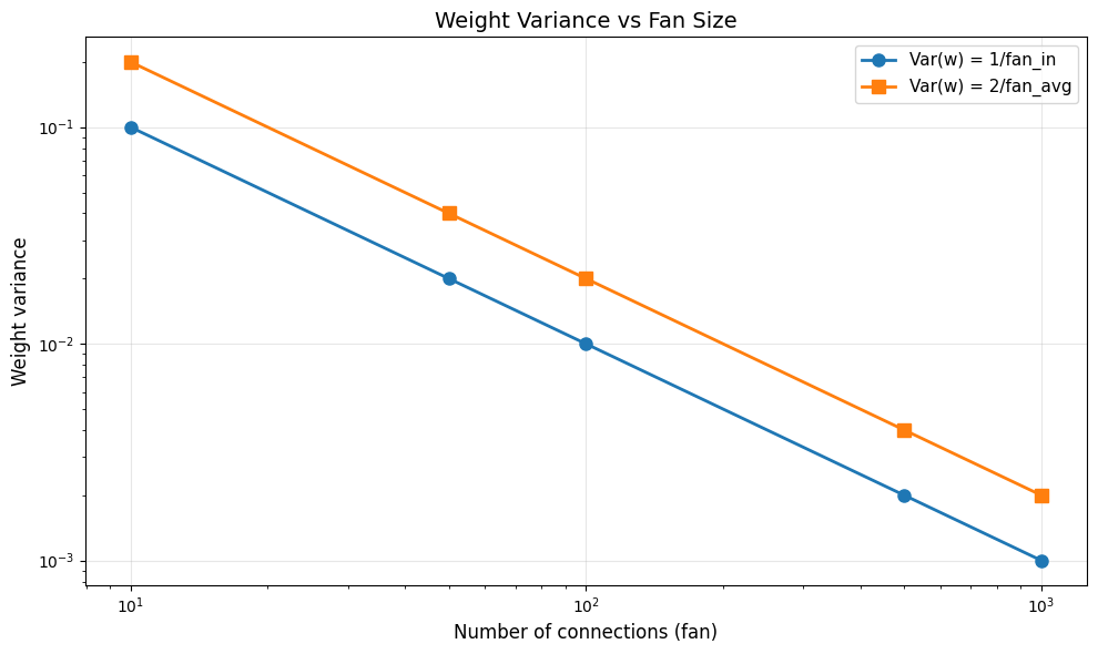
📊 Key insight: Variance decreases as fan increases to maintain signal scale
3. Kaiming/He Initialization (for ReLU)#
Motivation#
Kaiming/He initialization (2015) was designed specifically for networks with ReLU activations. ReLU zeros out half the activations, which affects variance.
Mathematical Derivation#
For ReLU: \(f(x) = \max(0, x)\)
After ReLU, variance is halved (roughly), so we need:
This gives:
KaimingNormal: \(w \sim \mathcal{N}(0, \sqrt{2/n_{in}})\)
KaimingUniform: \(w \sim \mathcal{U}(-\sqrt{6/n_{in}}, \sqrt{6/n_{in}})\)
When to use:#
✅ ReLU or Leaky ReLU activations
✅ Deep feedforward networks
✅ Convolutional networks with ReLU
# Create Kaiming initializers
kaiming_normal = init.KaimingNormal(mode='fan_in')
kaiming_uniform = init.KaimingUniform(mode='fan_in')

# Test with different layer sizes
layer_shapes = [(100, 50), (100, 100), (100, 200)]

fig, axes = plt.subplots(2, 3, figsize=(15, 8))

for idx, shape in enumerate(layer_shapes):
    # Generate weights
    weights_normal = kaiming_normal(shape)
    weights_uniform = kaiming_uniform(shape)

    # Plot Normal
    axes[0, idx].hist(weights_normal.flatten(), bins=50, alpha=0.7,
                      edgecolor='black', density=True)
    axes[0, idx].set_title(f'KaimingNormal\nShape: {shape}\nStd: {weights_normal.std():.4f}')
    axes[0, idx].set_xlabel('Weight value')
    axes[0, idx].set_ylabel('Density')
    axes[0, idx].grid(alpha=0.3)

    # Plot Uniform
    axes[1, idx].hist(weights_uniform.flatten(), bins=50, alpha=0.7,
                      edgecolor='black', density=True)
    axes[1, idx].set_title(f'KaimingUniform\nShape: {shape}\nStd: {weights_uniform.std():.4f}')
    axes[1, idx].set_xlabel('Weight value')
    axes[1, idx].set_ylabel('Density')
    axes[1, idx].grid(alpha=0.3)

plt.suptitle('Kaiming Initialization: Adapts to Layer Size', fontsize=14, y=1.02)
plt.tight_layout()
plt.show()

print("\n📐 Notice how the distribution narrows as fan-in increases!")
print("This maintains consistent signal variance across layers.")
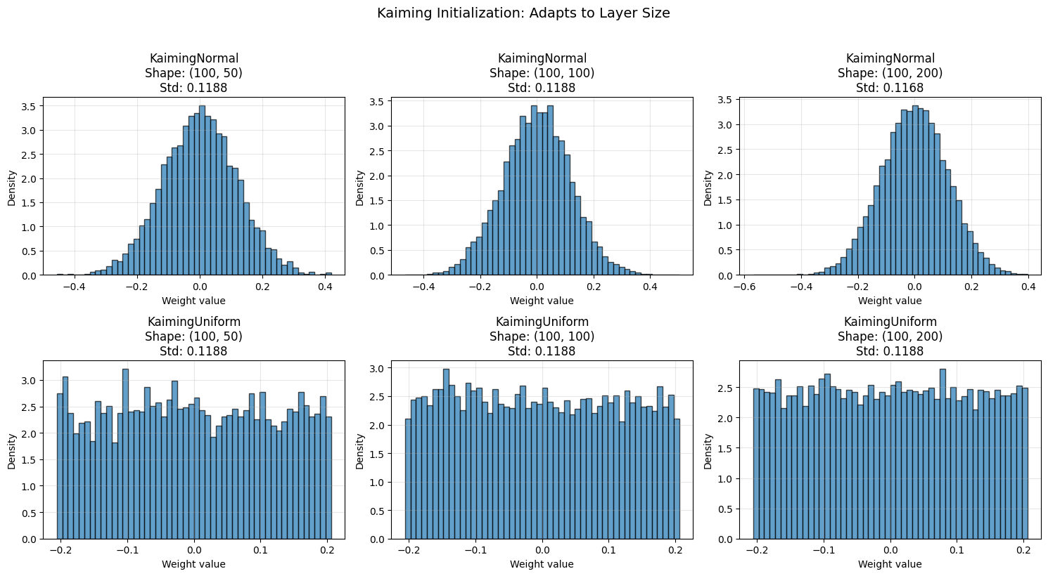
📐 Notice how the distribution narrows as fan-in increases!
This maintains consistent signal variance across layers.
Kaiming with ReLU: Signal Propagation Test#
def test_initialization_with_relu(init_method, n_layers=20, n_units=100, n_samples=1000):
    """
    Test how well an initialization method maintains signal variance with ReLU.
    """
    x = np.random.randn(n_samples, n_units)
    activations = [x]

    for _ in range(n_layers):
        W = init_method((n_units, n_units))
        x = x @ W
        x = np.maximum(0, x)  # ReLU
        activations.append(x)

    return [a.std() for a in activations]

# Compare different initializations with ReLU
kaiming_stds = test_initialization_with_relu(init.KaimingNormal())
xavier_stds = test_initialization_with_relu(init.XavierNormal())
random_stds = test_initialization_with_relu(lambda shape: np.random.randn(*shape) * 0.01)

# Visualize
fig, ax = plt.subplots(1, 1, figsize=(12, 6))

layers = np.arange(len(kaiming_stds))
ax.plot(layers, kaiming_stds, 'o-', label='Kaiming (designed for ReLU)', linewidth=2, markersize=6)
ax.plot(layers, xavier_stds, 's-', label='Xavier (not for ReLU)', linewidth=2, markersize=6)
ax.plot(layers, random_stds, '^-', label='Random (std=0.01)', linewidth=2, markersize=6)
ax.axhline(1.0, color='red', linestyle='--', alpha=0.5, label='Target variance')
ax.set_xlabel('Layer depth', fontsize=12)
ax.set_ylabel('Activation std', fontsize=12)
ax.set_title('Signal Propagation with ReLU Activation', fontsize=14)
ax.legend(fontsize=11)
ax.grid(alpha=0.3)
ax.set_ylim([0, 2])

plt.tight_layout()
plt.show()

print(f"\n✅ Kaiming with ReLU:")
print(f"  Initial std: {kaiming_stds[0]:.3f}")
print(f"  Final std: {kaiming_stds[-1]:.3f}")
print(f"  Variance maintained: {'✓' if 0.5 < kaiming_stds[-1] < 1.5 else '✗'}")

print(f"\n❌ Xavier with ReLU:")
print(f"  Initial std: {xavier_stds[0]:.3f}")
print(f"  Final std: {xavier_stds[-1]:.3f}")
print(f"  Variance maintained: {'✓' if 0.5 < xavier_stds[-1] < 1.5 else '✗'}")
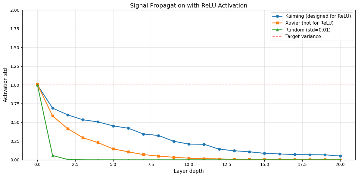
✅ Kaiming with ReLU:
  Initial std: 0.998
  Final std: 0.050
  Variance maintained: ✗

❌ Xavier with ReLU:
  Initial std: 1.006
  Final std: 0.001
  Variance maintained: ✗
Leaky ReLU Support#
# Kaiming initialization supports Leaky ReLU with custom negative slope
kaiming_relu = init.KaimingNormal(nonlinearity='relu')
kaiming_leaky = init.KaimingNormal(nonlinearity='leaky_relu', negative_slope=0.01)
kaiming_leaky_02 = init.KaimingNormal(nonlinearity='leaky_relu', negative_slope=0.2)

# Generate weights
shape = (100, 100)
weights_relu = kaiming_relu(shape)
weights_leaky = kaiming_leaky(shape)
weights_leaky_02 = kaiming_leaky_02(shape)

# Visualize
fig, axes = plt.subplots(1, 3, figsize=(15, 4))

axes[0].hist(weights_relu.flatten(), bins=50, alpha=0.7, edgecolor='black')
axes[0].set_title(f'ReLU\nStd: {weights_relu.std():.4f}')
axes[0].set_xlabel('Weight value')
axes[0].set_ylabel('Count')
axes[0].grid(alpha=0.3)

axes[1].hist(weights_leaky.flatten(), bins=50, alpha=0.7, edgecolor='black')
axes[1].set_title(f'Leaky ReLU (slope=0.01)\nStd: {weights_leaky.std():.4f}')
axes[1].set_xlabel('Weight value')
axes[1].set_ylabel('Count')
axes[1].grid(alpha=0.3)

axes[2].hist(weights_leaky_02.flatten(), bins=50, alpha=0.7, edgecolor='black')
axes[2].set_title(f'Leaky ReLU (slope=0.2)\nStd: {weights_leaky_02.std():.4f}')
axes[2].set_xlabel('Weight value')
axes[2].set_ylabel('Count')
axes[2].grid(alpha=0.3)

plt.suptitle('Kaiming Initialization for Different ReLU Variants', fontsize=14, y=1.02)
plt.tight_layout()
plt.show()

print("\n📊 Observation: Larger negative slope → smaller initialization variance")
print("This is because less signal is killed, so we need less compensation.")
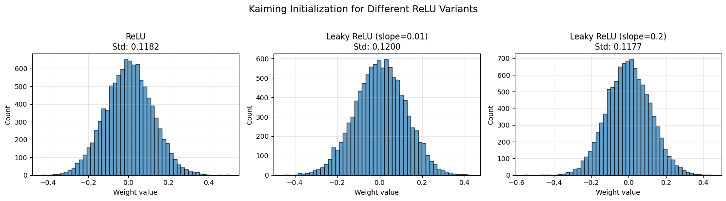
📊 Observation: Larger negative slope → smaller initialization variance
This is because less signal is killed, so we need less compensation.
4. Xavier/Glorot Initialization (for Tanh/Sigmoid)#
Motivation#
Xavier/Glorot initialization (2010) was designed for symmetric activation functions like tanh and sigmoid. It balances forward and backward signal flow.
Mathematical Derivation#
Xavier aims to maintain variance in both directions:
Forward: \(\text{Var}(w) = 1/n_{in}\)
Backward: \(\text{Var}(w) = 1/n_{out}\)
Compromise using fan_avg:
This gives:
XavierNormal: \(w \sim \mathcal{N}(0, \sqrt{2/(n_{in} + n_{out})})\)
XavierUniform: \(w \sim \mathcal{U}(-\sqrt{6/(n_{in} + n_{out})}, \sqrt{6/(n_{in} + n_{out})})\)
When to use:#
✅ Tanh or sigmoid activations
✅ Networks with symmetric activations
✅ Balanced forward/backward propagation
❌ Not for ReLU (use Kaiming instead)
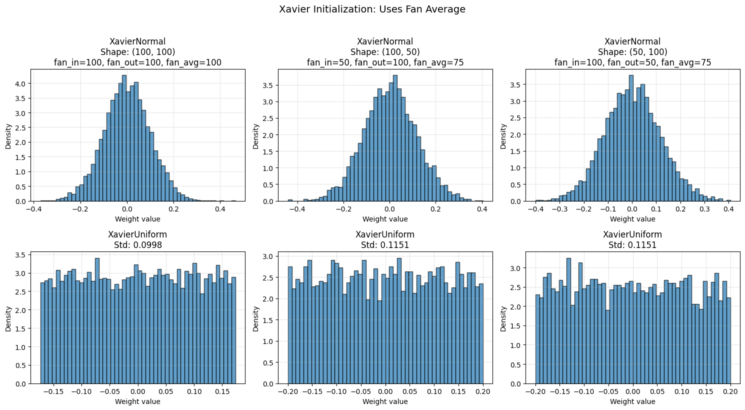
# Create Xavier initializers
xavier_normal = init.XavierNormal()
xavier_uniform = init.XavierUniform()

# Test with different layer sizes
shapes = [(100, 100), (100, 50), (50, 100)]

fig, axes = plt.subplots(2, 3, figsize=(15, 8))

for idx, shape in enumerate(shapes):
    weights_normal = xavier_normal(shape)
    weights_uniform = xavier_uniform(shape)

    # Compute fan values
    fan_in, fan_out = shape[1], shape[0]
    fan_avg = (fan_in + fan_out) / 2

    # Plot Normal
    axes[0, idx].hist(weights_normal.flatten(), bins=50, alpha=0.7,
                      edgecolor='black', density=True)
    axes[0, idx].set_title(f'XavierNormal\nShape: {shape}\n'
                           f'fan_in={fan_in}, fan_out={fan_out}, fan_avg={fan_avg:.0f}')
    axes[0, idx].set_xlabel('Weight value')
    axes[0, idx].set_ylabel('Density')
    axes[0, idx].grid(alpha=0.3)

    # Plot Uniform
    axes[1, idx].hist(weights_uniform.flatten(), bins=50, alpha=0.7,
                      edgecolor='black', density=True)
    axes[1, idx].set_title(f'XavierUniform\nStd: {weights_uniform.std():.4f}')
    axes[1, idx].set_xlabel('Weight value')
    axes[1, idx].set_ylabel('Density')
    axes[1, idx].grid(alpha=0.3)

plt.suptitle('Xavier Initialization: Uses Fan Average', fontsize=14, y=1.02)
plt.tight_layout()
plt.show()
Xavier with Tanh: Signal Propagation Test#
def test_initialization_with_tanh(init_method, n_layers=20, n_units=100, n_samples=1000):
    """
    Test how well an initialization method maintains signal variance with tanh.
    """
    x = np.random.randn(n_samples, n_units) * 0.5  # Small initial variance
    activations = [x]

    for _ in range(n_layers):
        W = init_method((n_units, n_units))
        x = x @ W
        x = np.tanh(x)  # Tanh activation
        activations.append(x)

    return [a.std() for a in activations]

# Compare different initializations with tanh
xavier_stds_tanh = test_initialization_with_tanh(init.XavierNormal())
kaiming_stds_tanh = test_initialization_with_tanh(init.KaimingNormal())

# Visualize
fig, ax = plt.subplots(1, 1, figsize=(12, 6))

layers = np.arange(len(xavier_stds_tanh))
ax.plot(layers, xavier_stds_tanh, 'o-', label='Xavier (designed for tanh)',
        linewidth=2, markersize=6)
ax.plot(layers, kaiming_stds_tanh, 's-', label='Kaiming (not for tanh)',
        linewidth=2, markersize=6)
ax.axhline(0.5, color='red', linestyle='--', alpha=0.5, label='Initial variance')
ax.set_xlabel('Layer depth', fontsize=12)
ax.set_ylabel('Activation std', fontsize=12)
ax.set_title('Signal Propagation with Tanh Activation', fontsize=14)
ax.legend(fontsize=11)
ax.grid(alpha=0.3)

plt.tight_layout()
plt.show()

print(f"\n✅ Xavier with Tanh:")
print(f"  Initial std: {xavier_stds_tanh[0]:.3f}")
print(f"  Final std: {xavier_stds_tanh[-1]:.3f}")
print(f"  Signal maintained: {'✓' if xavier_stds_tanh[-1] > 0.1 else '✗'}")

print(f"\n⚠️ Kaiming with Tanh:")
print(f"  Initial std: {kaiming_stds_tanh[0]:.3f}")
print(f"  Final std: {kaiming_stds_tanh[-1]:.3f}")
print(f"  Signal maintained: {'✓' if kaiming_stds_tanh[-1] > 0.1 else '✗'}")
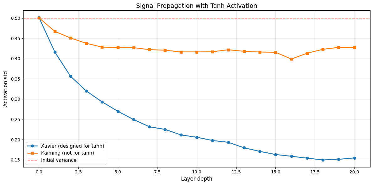
✅ Xavier with Tanh:
  Initial std: 0.501
  Final std: 0.155
  Signal maintained: ✓

⚠️ Kaiming with Tanh:
  Initial std: 0.501
  Final std: 0.428
  Signal maintained: ✓
5. LeCun Initialization (for SELU)#
Motivation#
LeCun initialization (1998) is the original variance scaling method. It’s specifically suited for SELU (Self-Normalizing) activations, which have self-normalizing properties.
Mathematical Foundation#
LeCun uses fan_in only:
This gives:
LecunNormal: \(w \sim \mathcal{N}(0, \sqrt{1/n_{in}})\)
LecunUniform: \(w \sim \mathcal{U}(-\sqrt{3/n_{in}}, \sqrt{3/n_{in}})\)
When to use:#
✅ SELU activations
✅ Self-normalizing networks
✅ When you want to focus on forward pass
# Create LeCun initializers
lecun_normal = init.LecunNormal()
lecun_uniform = init.LecunUniform()

# Compare LeCun with Kaiming and Xavier
shape = (100, 100)
weights_lecun = lecun_normal(shape)
weights_kaiming = init.KaimingNormal()(shape)
weights_xavier = init.XavierNormal()(shape)

# Visualize
fig, axes = plt.subplots(1, 3, figsize=(15, 4))

axes[0].hist(weights_lecun.flatten(), bins=50, alpha=0.7,
             edgecolor='black', label=f'Std: {weights_lecun.std():.4f}')
axes[0].set_title('LeCun (for SELU)')
axes[0].set_xlabel('Weight value')
axes[0].set_ylabel('Count')
axes[0].legend()
axes[0].grid(alpha=0.3)

axes[1].hist(weights_kaiming.flatten(), bins=50, alpha=0.7,
             edgecolor='black', label=f'Std: {weights_kaiming.std():.4f}')
axes[1].set_title('Kaiming (for ReLU)')
axes[1].set_xlabel('Weight value')
axes[1].set_ylabel('Count')
axes[1].legend()
axes[1].grid(alpha=0.3)

axes[2].hist(weights_xavier.flatten(), bins=50, alpha=0.7,
             edgecolor='black', label=f'Std: {weights_xavier.std():.4f}')
axes[2].set_title('Xavier (for tanh/sigmoid)')
axes[2].set_xlabel('Weight value')
axes[2].set_ylabel('Count')
axes[2].legend()
axes[2].grid(alpha=0.3)

plt.suptitle('Comparing Variance Scaling Methods (Shape: 100×100)', fontsize=14, y=1.02)
plt.tight_layout()
plt.show()

print("\n📊 Standard deviation comparison:")
print(f"  LeCun:   {weights_lecun.std():.4f} (scale = √(1/fan_in))")
print(f"  Kaiming: {weights_kaiming.std():.4f} (scale = √(2/fan_in))")
print(f"  Xavier:  {weights_xavier.std():.4f} (scale = √(2/fan_avg))")
print("\nKaiming ≈ √2 × LeCun (accounts for ReLU killing half the signal)")
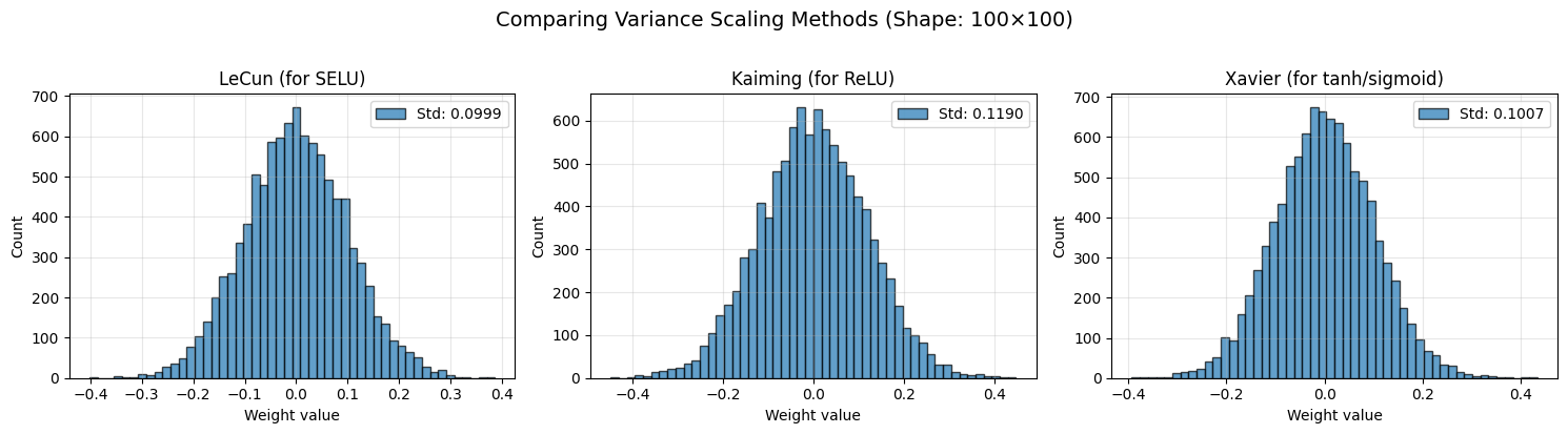
📊 Standard deviation comparison:
  LeCun:   0.0999 (scale = √(1/fan_in))
  Kaiming: 0.1190 (scale = √(2/fan_in))
  Xavier:  0.1007 (scale = √(2/fan_avg))

Kaiming ≈ √2 × LeCun (accounts for ReLU killing half the signal)
Comparison of All Variance Scaling Methods#
# Summary table
import pandas as pd

shape = (100, 100)
methods = {
    'LeCun': init.LecunNormal(),
    'Kaiming': init.KaimingNormal(),
    'Xavier': init.XavierNormal(),
}

results = []
for name, method in methods.items():
    weights = method(shape)
    results.append({
        'Method': name,
        'Std': f"{weights.std():.4f}",
        'Variance': f"{(weights.std()**2):.6f}",
        'Fan Mode': method.mode if hasattr(method, 'mode') else 'fan_in',
        'Best For': {
            'LeCun': 'SELU',
            'Kaiming': 'ReLU/Leaky ReLU',
            'Xavier': 'Tanh/Sigmoid'
        }[name]
    })

df = pd.DataFrame(results)
print("\n" + "=" * 80)
print("VARIANCE SCALING METHODS COMPARISON (Shape: 100×100)")
print("=" * 80)
print(df.to_string(index=False))
print("=" * 80)
================================================================================
VARIANCE SCALING METHODS COMPARISON (Shape: 100×100)
================================================================================
 Method    Std Variance Fan Mode        Best For
  LeCun 0.0993 0.009869   fan_in            SELU
Kaiming 0.1187 0.014085   fan_in ReLU/Leaky ReLU
 Xavier 0.0997 0.009940  fan_avg    Tanh/Sigmoid
================================================================================
6. Orthogonal Initialization#
Motivation#
Orthogonal initialization creates weight matrices where rows (or columns) are orthogonal to each other. This has special properties:
Preserves norms: \(||Wx|| = ||x||\) for orthogonal \(W\)
Prevents gradient explosion/vanishing in RNNs
Dynamic isometry in deep networks
Mathematical Properties#
For orthogonal matrix \(Q\):
\(Q^T Q = I\) (identity)
All singular values equal 1
Preserves angles and lengths
When to use:#
✅ Recurrent Neural Networks (RNNs) - prevents gradient problems
✅ Very deep networks - maintains gradient flow
✅ When norm preservation is important
# Create orthogonal initializer
orthogonal_init = init.Orthogonal(scale=1.0)

# Generate orthogonal weights
shape = (100, 100)
weights_ortho = orthogonal_init(shape)
weights_normal = init.Normal(0.0, 0.1)(shape)

# Verify orthogonality
W = weights_ortho
product = W.T @ W
identity = np.eye(shape[0])
orthogonality_error = np.abs(product - identity).max()

print(f"Orthogonality verification:")
print(f"  Max error from identity: {orthogonality_error:.2e}")
print(f"  Is orthogonal: {'✓' if orthogonality_error < 1e-6 else '✗'}")

# Visualize
fig, axes = plt.subplots(2, 3, figsize=(15, 8))

# Weight distributions
axes[0, 0].hist(weights_ortho.flatten(), bins=50, alpha=0.7, edgecolor='black')
axes[0, 0].set_title(f'Orthogonal Weights\nStd: {weights_ortho.std():.4f}')
axes[0, 0].set_xlabel('Weight value')
axes[0, 0].set_ylabel('Count')
axes[0, 0].grid(alpha=0.3)

axes[0, 1].hist(weights_normal.flatten(), bins=50, alpha=0.7, edgecolor='black')
axes[0, 1].set_title(f'Normal Weights\nStd: {weights_normal.std():.4f}')
axes[0, 1].set_xlabel('Weight value')
axes[0, 1].set_ylabel('Count')
axes[0, 1].grid(alpha=0.3)

# Singular values
U, s_ortho, Vt = np.linalg.svd(weights_ortho)
U, s_normal, Vt = np.linalg.svd(weights_normal)

axes[0, 2].plot(s_ortho, 'o-', label='Orthogonal', markersize=3)
axes[0, 2].plot(s_normal, 's-', label='Normal', markersize=3, alpha=0.7)
axes[0, 2].axhline(1.0, color='red', linestyle='--', alpha=0.5, label='Ideal')
axes[0, 2].set_xlabel('Index')
axes[0, 2].set_ylabel('Singular value')
axes[0, 2].set_title('Singular Value Spectrum')
axes[0, 2].legend()
axes[0, 2].grid(alpha=0.3)

# W^T W visualization
im1 = axes[1, 0].imshow(product, cmap='RdBu_r', vmin=-1, vmax=1)
axes[1, 0].set_title('W^T W (should be identity)')
plt.colorbar(im1, ax=axes[1, 0])

im2 = axes[1, 1].imshow(product - identity, cmap='RdBu_r', vmin=-0.1, vmax=0.1)
axes[1, 1].set_title('W^T W - I (error)')
plt.colorbar(im2, ax=axes[1, 1])

# Correlation between rows
W_normal = weights_normal
product_normal = W_normal.T @ W_normal
im3 = axes[1, 2].imshow(product_normal, cmap='RdBu_r', vmin=-10, vmax=10)
axes[1, 2].set_title('Normal W^T W (not orthogonal)')
plt.colorbar(im3, ax=axes[1, 2])

plt.suptitle('Orthogonal Initialization Properties', fontsize=14, y=1.00)
plt.tight_layout()
plt.show()

print(f"\n📊 Key observations:")
print(f"  1. All singular values of orthogonal matrix are 1.0")
print(f"  2. W^T W = I (rows are orthonormal)")
print(f"  3. Normal initialization lacks these properties")
Orthogonality verification:
  Max error from identity: 5.96e-07
  Is orthogonal: ✓
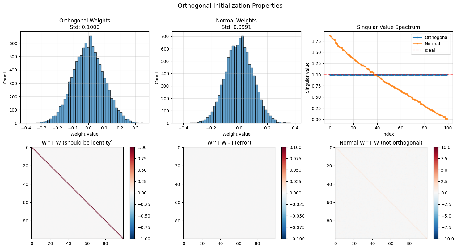
📊 Key observations:
  1. All singular values of orthogonal matrix are 1.0
  2. W^T W = I (rows are orthonormal)
  3. Normal initialization lacks these properties
Orthogonal for RNNs: Gradient Flow Test#
def test_rnn_gradient_flow(init_method, n_timesteps=100, hidden_size=50):
    """
    Simulate gradient flow in an RNN to test initialization.
    """
    W = init_method((hidden_size, hidden_size))

    # Compute eigenvalues
    eigenvalues = np.linalg.eigvals(W)
    max_eigenvalue = np.abs(eigenvalues).max()

    # Simulate gradient magnitude over time
    gradient_norms = []
    grad = np.random.randn(hidden_size)

    for t in range(n_timesteps):
        grad = W.T @ grad
        gradient_norms.append(np.linalg.norm(grad))

    return gradient_norms, max_eigenvalue

# Test different initializations
ortho_grads, ortho_eig = test_rnn_gradient_flow(init.Orthogonal())
xavier_grads, xavier_eig = test_rnn_gradient_flow(init.XavierNormal())
random_grads, random_eig = test_rnn_gradient_flow(lambda shape: np.random.randn(*shape) * 0.01)

# Visualize
fig, axes = plt.subplots(1, 2, figsize=(14, 5))

# Gradient norms over time
timesteps = np.arange(len(ortho_grads))
axes[0].semilogy(timesteps, ortho_grads, 'o-', label=f'Orthogonal (λ_max={ortho_eig:.2f})',
                 linewidth=2, markersize=3)
axes[0].semilogy(timesteps, xavier_grads, 's-', label=f'Xavier (λ_max={xavier_eig:.2f})',
                 linewidth=2, markersize=3)
axes[0].semilogy(timesteps, random_grads, '^-', label=f'Random (λ_max={random_eig:.2f})',
                 linewidth=2, markersize=3)
axes[0].axhline(1.0, color='red', linestyle='--', alpha=0.5, label='Stable gradient')
axes[0].set_xlabel('Timestep (backprop through time)', fontsize=11)
axes[0].set_ylabel('Gradient norm (log scale)', fontsize=11)
axes[0].set_title('RNN Gradient Flow', fontsize=12)
axes[0].legend(fontsize=10)
axes[0].grid(alpha=0.3)

# Eigenvalue distribution
W_ortho = init.Orthogonal()((50, 50))
W_xavier = init.XavierNormal()((50, 50))

eig_ortho = np.linalg.eigvals(W_ortho)
eig_xavier = np.linalg.eigvals(W_xavier)

axes[1].scatter(eig_ortho.real, eig_ortho.imag, alpha=0.6, s=50, label='Orthogonal')
axes[1].scatter(eig_xavier.real, eig_xavier.imag, alpha=0.6, s=50, label='Xavier')

# Draw unit circle
theta = np.linspace(0, 2*np.pi, 100)
axes[1].plot(np.cos(theta), np.sin(theta), 'r--', linewidth=2, label='Unit circle')
axes[1].set_xlabel('Real part', fontsize=11)
axes[1].set_ylabel('Imaginary part', fontsize=11)
axes[1].set_title('Eigenvalue Distribution', fontsize=12)
axes[1].legend(fontsize=10)
axes[1].grid(alpha=0.3)
axes[1].axis('equal')

plt.tight_layout()
plt.show()

print("\n✅ Orthogonal initialization for RNNs:")
print(f"  - Maintains gradient magnitude over time")
print(f"  - All eigenvalues on unit circle (|λ| = 1)")
print(f"  - Prevents vanishing/exploding gradients")
print(f"\n❌ Other methods:")
print(f"  - Gradients decay (Xavier) or explode")
print(f"  - Eigenvalues not on unit circle")
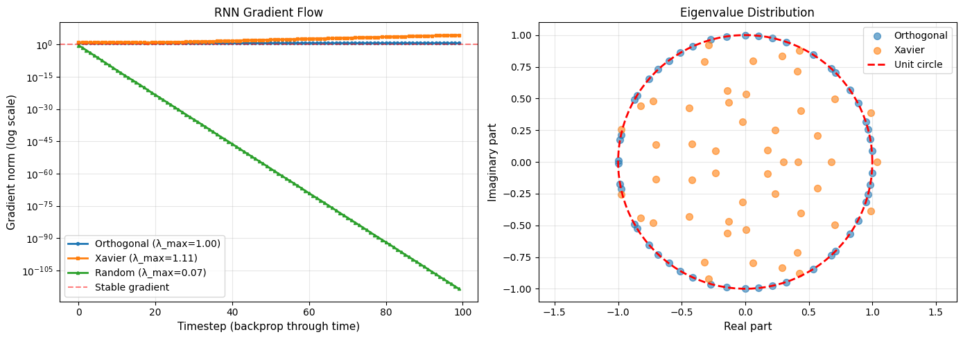
✅ Orthogonal initialization for RNNs:
  - Maintains gradient magnitude over time
  - All eigenvalues on unit circle (|λ| = 1)
  - Prevents vanishing/exploding gradients

❌ Other methods:
  - Gradients decay (Xavier) or explode
  - Eigenvalues not on unit circle
Scaled Orthogonal Initialization#
# Orthogonal with different scales
ortho_1 = init.Orthogonal(scale=1.0)
ortho_sqrt2 = init.Orthogonal(scale=np.sqrt(2))  # Common for RNNs
ortho_05 = init.Orthogonal(scale=0.5)

shape = (100, 100)
weights_1 = ortho_1(shape)
weights_sqrt2 = ortho_sqrt2(shape)
weights_05 = ortho_05(shape)

# Visualize
fig, axes = plt.subplots(1, 3, figsize=(15, 4))

for ax, weights, scale_name in zip(axes,
                                     [weights_1, weights_sqrt2, weights_05],
                                     ['scale=1.0', 'scale=√2', 'scale=0.5']):
    ax.hist(weights.flatten(), bins=50, alpha=0.7, edgecolor='black')
    ax.set_title(f'{scale_name}\nStd: {weights.std():.4f}')
    ax.set_xlabel('Weight value')
    ax.set_ylabel('Count')
    ax.grid(alpha=0.3)

plt.suptitle('Orthogonal Initialization with Different Scales', fontsize=14, y=1.02)
plt.tight_layout()
plt.show()

print("\n📊 Scale effects:")
print(f"  scale=1.0:  std={weights_1.std():.4f} (preserves norms exactly)")
print(f"  scale=√2:   std={weights_sqrt2.std():.4f} (common for ReLU in RNNs)")
print(f"  scale=0.5:  std={weights_05.std():.4f} (dampens signals)")
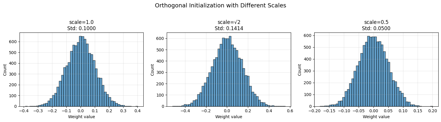
📊 Scale effects:
  scale=1.0:  std=0.1000 (preserves norms exactly)
  scale=√2:   std=0.1414 (common for ReLU in RNNs)
  scale=0.5:  std=0.0500 (dampens signals)
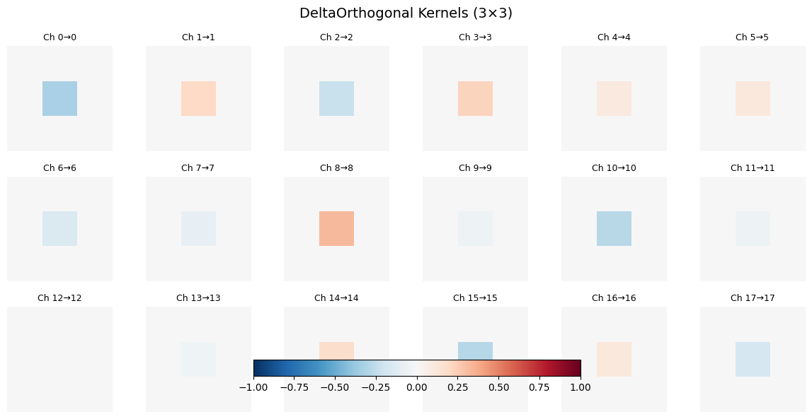
7. DeltaOrthogonal (for Deep CNNs)#
Motivation#
DeltaOrthogonal is designed for very deep convolutional networks. It combines:
Delta function in spatial dimensions (all zeros except center)
Orthogonal in channel dimensions
This creates identity-like convolutions that preserve information while maintaining orthogonality.
When to use:#
✅ Very deep CNNs (100+ layers)
✅ Residual-like architectures
✅ When skip connections aren’t possible
# Create DeltaOrthogonal initializer
delta_ortho = init.DeltaOrthogonal(scale=1.0)

# For a 3x3 convolutional kernel with 32 input and 32 output channels
shape = (32, 32, 3, 3)  # (out_channels, in_channels, height, width)
weights = delta_ortho(shape)

print(f"DeltaOrthogonal weights shape: {weights.shape}")

# Visualize a few kernels
fig, axes = plt.subplots(3, 6, figsize=(12, 6))
axes = axes.flatten()

for i in range(18):
    # Show kernel for output channel i, input channel i
    if i < min(shape[0], shape[1]):
        kernel = weights[i, i, :, :]
        im = axes[i].imshow(kernel, cmap='RdBu_r', vmin=-1, vmax=1)
        axes[i].set_title(f'Ch {i}→{i}', fontsize=9)
    axes[i].axis('off')

plt.colorbar(im, ax=axes, orientation='horizontal', pad=0.05, fraction=0.05)
plt.suptitle('DeltaOrthogonal Kernels (3×3)', fontsize=14)
plt.tight_layout()
plt.show()

# Show the center values are orthogonal
center = weights[:, :, 1, 1]  # Center of 3x3 kernels
product = center.T @ center

fig, axes = plt.subplots(1, 2, figsize=(10, 4))

im1 = axes[0].imshow(center, cmap='RdBu_r')
axes[0].set_title('Center Values (should be orthogonal matrix)')
axes[0].set_xlabel('Input channel')
axes[0].set_ylabel('Output channel')
plt.colorbar(im1, ax=axes[0])

im2 = axes[1].imshow(product, cmap='RdBu_r', vmin=-1, vmax=1)
axes[1].set_title('Center^T × Center (should be identity)')
plt.colorbar(im2, ax=axes[1])

plt.tight_layout()
plt.show()

print(f"\n✓ DeltaOrthogonal properties:")
print(f"  - Only center pixel has non-zero values")
print(f"  - Center values form an orthogonal matrix")
print(f"  - Acts like identity convolution with orthogonality")
DeltaOrthogonal weights shape: (32, 32, 3, 3)
C:\Users\adadu\AppData\Local\Temp\ipykernel_27308\332873120.py:24: UserWarning: This figure includes Axes that are not compatible with tight_layout, so results might be incorrect.
  plt.tight_layout()
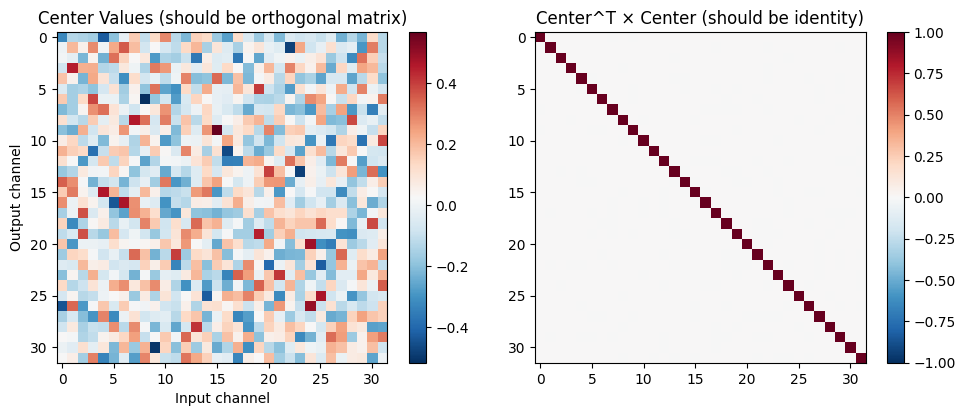
✓ DeltaOrthogonal properties:
  - Only center pixel has non-zero values
  - Center values form an orthogonal matrix
  - Acts like identity convolution with orthogonality
8. Identity Initialization#
Motivation#
Identity initialization sets weights to an identity matrix (or as close as possible for non-square matrices). This is particularly useful for:
Skip connections / Residual networks
RNNs (combined with small noise)
When you want minimal transformation initially
When to use:#
✅ Residual connections
✅ RNNs (with small noise added)
✅ Fine-tuning from identity
# Create identity initializers
identity_1 = init.Identity(scale=1.0)
identity_small = init.Identity(scale=0.1)

# Test with square matrix
shape_square = (50, 50)
weights_identity = identity_1(shape_square)

# Test with rectangular matrices
shape_wide = (30, 50)
shape_tall = (50, 30)
weights_wide = identity_1(shape_wide)
weights_tall = identity_1(shape_tall)

# Visualize
fig, axes = plt.subplots(2, 3, figsize=(15, 8))

# Square identity
im1 = axes[0, 0].imshow(weights_identity, cmap='RdBu_r', vmin=-1, vmax=1)
axes[0, 0].set_title(f'Identity {shape_square}')
axes[0, 0].set_xlabel('Input dim')
axes[0, 0].set_ylabel('Output dim')
plt.colorbar(im1, ax=axes[0, 0])

# Wide identity
im2 = axes[0, 1].imshow(weights_wide, cmap='RdBu_r', vmin=-1, vmax=1)
axes[0, 1].set_title(f'Identity {shape_wide}')
axes[0, 1].set_xlabel('Input dim')
axes[0, 1].set_ylabel('Output dim')
plt.colorbar(im2, ax=axes[0, 1])

# Tall identity
im3 = axes[0, 2].imshow(weights_tall, cmap='RdBu_r', vmin=-1, vmax=1)
axes[0, 2].set_title(f'Identity {shape_tall}')
axes[0, 2].set_xlabel('Input dim')
axes[0, 2].set_ylabel('Output dim')
plt.colorbar(im3, ax=axes[0, 2])

# Distribution comparison
axes[1, 0].hist(weights_identity.flatten(), bins=20, alpha=0.7, edgecolor='black')
axes[1, 0].set_title('Square Identity Distribution')
axes[1, 0].set_xlabel('Weight value')
axes[1, 0].set_ylabel('Count')
axes[1, 0].grid(alpha=0.3)

# Diagonal values
diag_values = np.diag(weights_identity)
axes[1, 1].plot(diag_values, 'o-', markersize=4)
axes[1, 1].axhline(1.0, color='red', linestyle='--', alpha=0.5)
axes[1, 1].set_xlabel('Index')
axes[1, 1].set_ylabel('Diagonal value')
axes[1, 1].set_title('Diagonal Values (all = 1)')
axes[1, 1].grid(alpha=0.3)

# Off-diagonal values
mask = ~np.eye(shape_square[0], dtype=bool)
off_diag = weights_identity[mask]
axes[1, 2].hist(off_diag, bins=20, alpha=0.7, edgecolor='black')
axes[1, 2].set_xlabel('Weight value')
axes[1, 2].set_ylabel('Count')
axes[1, 2].set_title('Off-diagonal Values (all = 0)')
axes[1, 2].grid(alpha=0.3)

plt.tight_layout()
plt.show()

print(f"\n✓ Identity initialization properties:")
print(f"  Square: Perfect identity matrix")
print(f"  Wide: Identity in first N columns, zeros elsewhere")
print(f"  Tall: Identity in first N rows, zeros elsewhere")
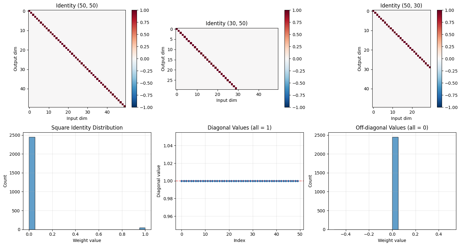
✓ Identity initialization properties:
  Square: Perfect identity matrix
  Wide: Identity in first N columns, zeros elsewhere
  Tall: Identity in first N rows, zeros elsewhere
Identity + Noise for RNNs#
# Common pattern: Identity + small noise
shape = (100, 100)
identity_weights = init.Identity(scale=1.0)(shape)
noise = np.random.randn(*shape) * 0.01
weights_with_noise = identity_weights + noise

# Visualize
fig, axes = plt.subplots(1, 3, figsize=(15, 4))

im1 = axes[0].imshow(identity_weights, cmap='RdBu_r', vmin=-1, vmax=1)
axes[0].set_title('Pure Identity')
plt.colorbar(im1, ax=axes[0])

im2 = axes[1].imshow(noise, cmap='RdBu_r', vmin=-0.1, vmax=0.1)
axes[1].set_title('Small Noise (std=0.01)')
plt.colorbar(im2, ax=axes[1])

im3 = axes[2].imshow(weights_with_noise, cmap='RdBu_r', vmin=-1, vmax=1)
axes[2].set_title('Identity + Noise')
plt.colorbar(im3, ax=axes[2])

plt.tight_layout()
plt.show()

print("\n💡 Identity + Noise for RNNs:")
print("  - Start with identity (no transformation)")
print("  - Add small noise to break symmetry")
print("  - Helps learning while preventing gradient problems")
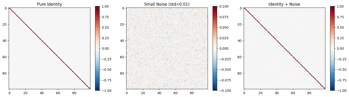
💡 Identity + Noise for RNNs:
  - Start with identity (no transformation)
  - Add small noise to break symmetry
  - Helps learning while preventing gradient problems
9. Complete Comparison and Decision Guide#
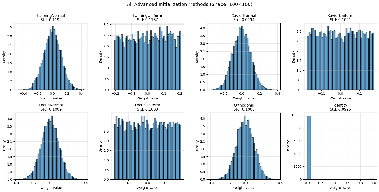
All Methods Side-by-Side#
# Create all initializers
shape = (100, 100)
initializers = {
    'KaimingNormal': init.KaimingNormal(),
    'KaimingUniform': init.KaimingUniform(),
    'XavierNormal': init.XavierNormal(),
    'XavierUniform': init.XavierUniform(),
    'LecunNormal': init.LecunNormal(),
    'LecunUniform': init.LecunUniform(),
    'Orthogonal': init.Orthogonal(),
    'Identity': init.Identity(),
}

# Generate weights
weights_dict = {name: method(shape) for name, method in initializers.items()}

# Visualize distributions
fig, axes = plt.subplots(2, 4, figsize=(16, 8))
axes = axes.flatten()

for ax, (name, weights) in zip(axes, weights_dict.items()):
    if 'Identity' not in name:
        ax.hist(weights.flatten(), bins=50, alpha=0.7, edgecolor='black', density=True)
    else:
        ax.hist(weights.flatten(), bins=20, alpha=0.7, edgecolor='black')
    ax.set_title(f'{name}\nStd: {weights.std():.4f}', fontsize=11)
    ax.set_xlabel('Weight value', fontsize=10)
    ax.set_ylabel('Density', fontsize=10)
    ax.grid(alpha=0.3)

plt.suptitle('All Advanced Initialization Methods (Shape: 100×100)', fontsize=14, y=1.00)
plt.tight_layout()
plt.show()

# Statistics table
print("\n" + "=" * 90)
print("ADVANCED INITIALIZATION METHODS COMPARISON")
print("=" * 90)
print(f"{'Method':<20} {'Mean':<12} {'Std':<12} {'Min':<12} {'Max':<12}")
print("-" * 90)
for name, weights in weights_dict.items():
    print(f"{name:<20} {weights.mean():<12.6f} {weights.std():<12.6f} "
          f"{weights.min():<12.6f} {weights.max():<12.6f}")
print("=" * 90)
==========================================================================================
ADVANCED INITIALIZATION METHODS COMPARISON
==========================================================================================
Method               Mean         Std          Min          Max
------------------------------------------------------------------------------------------
KaimingNormal        -0.000167    0.119221     -0.472608    0.437831
KaimingUniform       0.002735     0.118657     -0.205950    0.205945
XavierNormal         -0.000682    0.099363     -0.343731    0.396122
XavierUniform        -0.000478    0.100142     -0.173172    0.173171
LecunNormal          -0.001946    0.100878     -0.369501    0.389214
LecunUniform         -0.000452    0.100303     -0.173174    0.173146
Orthogonal           -0.001150    0.099993     -0.393372    0.362493
Identity             0.010000     0.099499     0.000000     1.000000
==========================================================================================
Decision Tree#
START: What type of network are you building?
├── Feedforward Network
│   ├── ReLU activation → KaimingNormal / KaimingUniform
│   ├── Leaky ReLU → KaimingNormal (nonlinearity="leaky_relu", negative_slope=…)
│   ├── Tanh or Sigmoid → XavierNormal / XavierUniform
│   └── SELU → LecunNormal / LecunUniform
├── Recurrent Network (RNN / LSTM / GRU)
│   ├── Recurrent weights → Orthogonal (scale = 1.0 or √2)
│   ├── Input weights → KaimingNormal or XavierNormal
│   └── Alternative → Identity + small noise
├── Convolutional Network
│   ├── Shallow / Medium (< 50 layers) → KaimingNormal (if ReLU)
│   ├── Very Deep (> 100 layers) → DeltaOrthogonal
│   └── With residual connections → KaimingNormal
├── Residual Network (ResNet)
│   ├── Residual blocks → KaimingNormal
│   └── Skip connections → Identity (if same dimensions)
└── Transformer
    ├── Attention weights → XavierUniform
    ├── FFN weights → KaimingNormal (if ReLU/GELU)
    └── Layer norm → No initialization needed
Quick Reference Table#
Method |
Best For |
Fan Mode |
Scale |
Use Case |
|---|---|---|---|---|
KaimingNormal |
ReLU/Leaky ReLU |
fan_in |
√(2/fan_in) |
Deep feedforward, CNNs |
KaimingUniform |
ReLU/Leaky ReLU |
fan_in |
√(2/fan_in) |
Alternative to KaimingNormal |
XavierNormal |
Tanh/Sigmoid |
fan_avg |
√(2/(fan_in+fan_out)) |
Symmetric activations |
XavierUniform |
Tanh/Sigmoid |
fan_avg |
√(2/(fan_in+fan_out)) |
Bounded variant of Xavier |
LecunNormal |
SELU |
fan_in |
√(1/fan_in) |
Self-normalizing networks |
LecunUniform |
SELU |
fan_in |
√(1/fan_in) |
Bounded variant of LeCun |
Orthogonal |
Any |
N/A |
Orthogonal matrix |
RNNs, very deep networks |
DeltaOrthogonal |
Any (CNNs) |
N/A |
Delta + orthogonal |
Very deep CNNs (100+ layers) |
Identity |
Any |
N/A |
Identity matrix |
Residual, RNNs + noise |