
Tutorial 4: Learning Rate Scheduling Strategies#
Difficulty: Intermediate
Duration: 30-40 minutes
Prerequisites: Tutorial 3 completion
Learning Objectives#
Implement various learning rate schedules
Combine optimizers with schedulers
Understand when to use different scheduling strategies
Monitor and visualize learning rate changes
Topics Covered#
Basic schedulers
StepLR: Step-wise decay
ExponentialLR: Exponential decay
MultiStepLR: Custom milestone-based decay
Advanced schedulers
CosineAnnealingLR: Cosine annealing
CyclicLR: Cyclic learning rates
OneCycleLR: Super-convergence training
Adaptive scheduling
ReduceLROnPlateau: Metric-based adaptation
WarmupScheduler: Gradual warmup strategies
Scheduler composition
ChainedScheduler: Sequential scheduling
SequentialLR: Phase-based scheduling
import time

import brainstate
import braintools

import jax
import jax.numpy as jnp
import matplotlib.pyplot as plt
import numpy as np
1. Setting up the Model and Data#
We’ll use a CNN model for this tutorial to demonstrate learning rate scheduling on a more complex architecture.
class SimpleNet(brainstate.nn.Module):
    def __init__(self, num_classes=10):
        super().__init__()
        self.fc1 = brainstate.nn.Linear(784, 128)
        self.fc2 = brainstate.nn.Linear(128, num_classes)

    def __call__(self, x):
        x = self.fc1(x)
        x = jax.nn.relu(x)
        x = self.fc2(x)
        return x
# Create synthetic CIFAR-like data
def create_synthetic_data(n_train=5000, n_val=1000, seed=42):
    """Create synthetic image classification data."""
    with brainstate.random.seed_context(seed):
        # Training data
        X_train = brainstate.random.normal(size=(n_train, 784)) * 0.5
        y_train = brainstate.random.randint(0, 10, size=(n_train,))

        # Validation data
        X_val = brainstate.random.normal(size=(n_val, 784)) * 0.5
        y_val = brainstate.random.randint(0, 10, size=(n_val,))

    return X_train, y_train, X_val, y_val


X_train, y_train, X_val, y_val = create_synthetic_data()
print(f"Training data: {X_train.shape}, Validation data: {X_val.shape}")
Training data: (5000, 784), Validation data: (1000, 784)
2. Gradient Computation and Training Loop#
Following the style from the optax tutorial, we’ll define our training infrastructure.
def compute_loss_and_grads(model, X, y, param_states):
    """Compute loss and gradients following braintools style."""

    def loss_fn():
        # Forward pass
        logits = model(X)

        # Cross-entropy loss
        log_probs = jax.nn.log_softmax(logits, axis=-1)
        one_hot = jax.nn.one_hot(y, num_classes=10)
        loss = -jnp.mean(jnp.sum(one_hot * log_probs, axis=-1))

        return loss

    # Compute loss and gradients
    loss = loss_fn()
    grads = brainstate.transform.grad(loss_fn, grad_states=param_states)()

    # Compute accuracy
    logits = model(X)
    predictions = jnp.argmax(logits, axis=-1)
    accuracy = jnp.mean(predictions == y)

    return loss, grads, accuracy
def train_with_scheduler(
    model: brainstate.nn.Module,
    optimizer: braintools.optim.OptaxOptimizer,
    X_train, y_train, X_val, y_val,
    n_epochs=50,
    batch_size=128,
    verbose=True,
    track_lr=True
):
    """Train model with learning rate scheduling."""

    # Get parameter states
    param_states = braintools.optim.UniqueStateManager(
        model.states(brainstate.ParamState)
    ).to_pytree()

    # Initialize optimizer
    optimizer.register_trainable_weights(param_states)

    @brainstate.transform.jit
    def train_step(X_batch, y_batch):
        loss, grads, acc = compute_loss_and_grads(model, X_batch, y_batch, param_states)
        optimizer.update(grads)
        return loss, acc

    @brainstate.transform.jit
    def eval_step(X_batch, y_batch):
        loss, _, acc = compute_loss_and_grads(model, X_batch, y_batch, param_states)
        return loss, acc

    # Training history
    history = {
        'train_loss': [],
        'train_acc': [],
        'val_loss': [],
        'val_acc': [],
        'lr': [],
        'epoch_time': []
    }

    n_batches = len(X_train) // batch_size

    for epoch in range(n_epochs):
        epoch_start = time.time()

        # Shuffle training data
        perm = brainstate.random.permutation(len(X_train))
        X_train_shuffled = X_train[perm]
        y_train_shuffled = y_train[perm]

        # Training
        train_losses = []
        train_accs = []

        for batch_idx in range(n_batches):
            start_idx = batch_idx * batch_size
            end_idx = start_idx + batch_size
            X_batch = X_train_shuffled[start_idx:end_idx]
            y_batch = y_train_shuffled[start_idx:end_idx]

            loss, acc = train_step(X_batch, y_batch)
            train_losses.append(float(loss))
            train_accs.append(float(acc))

        # Validation
        val_loss, val_acc = eval_step(X_val, y_val)

        # Update learning rate scheduler
        optimizer.lr.step()

        # Track current learning rate
        if track_lr:
            current_lr = optimizer.lr.get_lr()[0]
        else:
            current_lr = 0.0

        # Record metrics
        history['train_loss'].append(np.mean(train_losses))
        history['train_acc'].append(np.mean(train_accs))
        history['val_loss'].append(float(val_loss))
        history['val_acc'].append(float(val_acc))
        history['lr'].append(current_lr)
        history['epoch_time'].append(time.time() - epoch_start)

        if verbose and (epoch + 1) % 10 == 0:
            print(
                f"Epoch {epoch + 1}/{n_epochs} - "
                f"Loss: {history['train_loss'][-1]:.4f}, "
                f"Acc: {history['train_acc'][-1]:.4f}, "
                f"Val Loss: {history['val_loss'][-1]:.4f}, "
                f"Val Acc: {history['val_acc'][-1]:.4f}, "
                f"LR: {current_lr:.6f}"
            )

    return history
3. Basic Learning Rate Schedulers#
Let’s implement and compare basic learning rate scheduling strategies.
3.1 Step Decay Scheduler#
# Create model with Step LR scheduler
model_step = SimpleNet()

# Step decay: reduce LR by gamma every step_size epochs
step_lr = braintools.optim.StepLR(
    base_lr=0.01,
    step_size=10,
    gamma=0.5,
    last_epoch=0
)

optimizer_step = braintools.optim.Adam(lr=step_lr)

print("Training with Step LR Decay...")
history_step = train_with_scheduler(
    model_step, optimizer_step,
    X_train, y_train, X_val, y_val,
    n_epochs=40, batch_size=128
)
Training with Step LR Decay...
Epoch 10/40 - Loss: 0.0030, Acc: 1.0000, Val Loss: 5.8856, Val Acc: 0.1010, LR: 0.005000
Epoch 20/40 - Loss: 0.0013, Acc: 1.0000, Val Loss: 6.1810, Val Acc: 0.1010, LR: 0.002500
Epoch 30/40 - Loss: 0.0010, Acc: 1.0000, Val Loss: 6.3180, Val Acc: 0.0990, LR: 0.001250
Epoch 40/40 - Loss: 0.0008, Acc: 1.0000, Val Loss: 6.3916, Val Acc: 0.0990, LR: 0.000625
3.2 Exponential Decay Scheduler#
# Create model with Exponential LR scheduler
model_exp = SimpleNet()

# Exponential decay: lr = init_lr * gamma^epoch
exp_lr = braintools.optim.ExponentialLR(
    base_lr=0.01,
    gamma=0.95,
    last_epoch=0
)

optimizer_exp = braintools.optim.Adam(lr=exp_lr)

print("Training with Exponential LR Decay...")
history_exp = train_with_scheduler(
    model_exp, optimizer_exp,
    X_train, y_train, X_val, y_val,
    n_epochs=40, batch_size=128
)
Training with Exponential LR Decay...
Epoch 10/40 - Loss: 0.0049, Acc: 1.0000, Val Loss: 5.5179, Val Acc: 0.1120, LR: 0.005987
Epoch 20/40 - Loss: 0.0019, Acc: 1.0000, Val Loss: 5.9411, Val Acc: 0.1130, LR: 0.003585
Epoch 30/40 - Loss: 0.0012, Acc: 1.0000, Val Loss: 6.1494, Val Acc: 0.1130, LR: 0.002146
Epoch 40/40 - Loss: 0.0009, Acc: 1.0000, Val Loss: 6.2729, Val Acc: 0.1140, LR: 0.001285
3.3 MultiStep Decay Scheduler#
# Create model with MultiStep LR scheduler
model_multistep = SimpleNet()

# MultiStep decay: reduce LR at specific milestones
multistep_lr = braintools.optim.MultiStepLR(
    base_lr=0.01,
    milestones=[10, 20, 30],
    gamma=0.3,
    last_epoch=0
)

optimizer_multistep = braintools.optim.Adam(lr=multistep_lr)

print("Training with MultiStep LR Decay...")
history_multistep = train_with_scheduler(
    model_multistep, optimizer_multistep,
    X_train, y_train, X_val, y_val,
    n_epochs=40, batch_size=128
)
Training with MultiStep LR Decay...
Epoch 10/40 - Loss: 0.0030, Acc: 1.0000, Val Loss: 5.8258, Val Acc: 0.1270, LR: 0.003000
Epoch 20/40 - Loss: 0.0017, Acc: 1.0000, Val Loss: 6.0254, Val Acc: 0.1250, LR: 0.000900
Epoch 30/40 - Loss: 0.0014, Acc: 1.0000, Val Loss: 6.0906, Val Acc: 0.1230, LR: 0.000270
Epoch 40/40 - Loss: 0.0013, Acc: 1.0000, Val Loss: 6.1144, Val Acc: 0.1240, LR: 0.000270
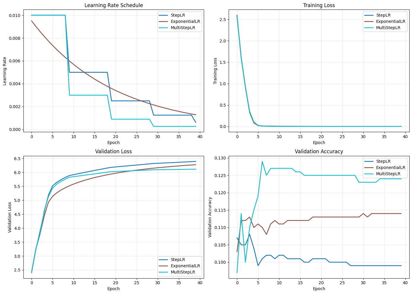
3.4 Visualizing Basic Schedulers#
def plot_lr_schedules(histories, names, colors=None):
    """Plot learning rate schedules and training curves."""
    if colors is None:
        colors = plt.cm.tab10(np.linspace(0, 1, len(histories)))

    fig, axes = plt.subplots(2, 2, figsize=(14, 10))

    # Learning rate over time
    ax = axes[0, 0]
    for history, name, color in zip(histories, names, colors):
        ax.plot(history['lr'], label=name, color=color, linewidth=2)
    ax.set_xlabel('Epoch')
    ax.set_ylabel('Learning Rate')
    ax.set_title('Learning Rate Schedule')
    ax.legend()
    ax.grid(True, alpha=0.3)

    # Training loss
    ax = axes[0, 1]
    for history, name, color in zip(histories, names, colors):
        ax.plot(history['train_loss'], label=name, color=color, linewidth=2)
    ax.set_xlabel('Epoch')
    ax.set_ylabel('Training Loss')
    ax.set_title('Training Loss')
    ax.legend()
    ax.grid(True, alpha=0.3)

    # Validation loss
    ax = axes[1, 0]
    for history, name, color in zip(histories, names, colors):
        ax.plot(history['val_loss'], label=name, color=color, linewidth=2)
    ax.set_xlabel('Epoch')
    ax.set_ylabel('Validation Loss')
    ax.set_title('Validation Loss')
    ax.legend()
    ax.grid(True, alpha=0.3)

    # Validation accuracy
    ax = axes[1, 1]
    for history, name, color in zip(histories, names, colors):
        ax.plot(history['val_acc'], label=name, color=color, linewidth=2)
    ax.set_xlabel('Epoch')
    ax.set_ylabel('Validation Accuracy')
    ax.set_title('Validation Accuracy')
    ax.legend()
    ax.grid(True, alpha=0.3)

    plt.tight_layout()
    plt.show()


# Compare basic schedulers
plot_lr_schedules(
    [history_step, history_exp, history_multistep],
    ['StepLR', 'ExponentialLR', 'MultiStepLR']
)
4. Advanced Learning Rate Schedulers#
Now let’s explore more sophisticated scheduling strategies.
4.1 Cosine Annealing Scheduler#
# Create model with Cosine Annealing scheduler
model_cosine = SimpleNet()

# Cosine annealing: smoothly decreases LR following cosine curve
cosine_lr = braintools.optim.CosineAnnealingLR(
    base_lr=0.01,
    T_max=20,  # Half period of cosine
    eta_min=0.0001,  # Minimum LR
    last_epoch=0
)

optimizer_cosine = braintools.optim.Adam(lr=cosine_lr)

print("Training with Cosine Annealing...")
history_cosine = train_with_scheduler(
    model_cosine, optimizer_cosine,
    X_train, y_train, X_val, y_val,
    n_epochs=40, batch_size=128
)
Training with Cosine Annealing...
Epoch 10/40 - Loss: 0.0042, Acc: 1.0000, Val Loss: 5.7146, Val Acc: 0.0970, LR: 0.005050
Epoch 20/40 - Loss: 0.0025, Acc: 1.0000, Val Loss: 5.9071, Val Acc: 0.0940, LR: 0.000100
Epoch 30/40 - Loss: 0.0018, Acc: 1.0000, Val Loss: 6.0856, Val Acc: 0.0950, LR: 0.005050
Epoch 40/40 - Loss: 0.0006, Acc: 1.0000, Val Loss: 6.6336, Val Acc: 0.0990, LR: 0.010000
4.2 Cyclic Learning Rate (CyclicLR)#
# Create model with Cyclic LR scheduler
model_cyclic = SimpleNet()

# Cyclic LR: oscillates between base_lr and max_lr
cyclic_lr = braintools.optim.CyclicLR(
    base_lr=0.001,
    max_lr=0.01,
    step_size_up=5,  # Epochs to increase LR
    step_size_down=5,  # Epochs to decrease LR
    mode='triangular2',  # Halve max_lr after each cycle
    last_epoch=0
)

optimizer_cyclic = braintools.optim.SGD(lr=cyclic_lr, momentum=0.9)

print("Training with Cyclic LR...")
history_cyclic = train_with_scheduler(
    model_cyclic, optimizer_cyclic,
    X_train, y_train, X_val, y_val,
    n_epochs=40, batch_size=128
)
Training with Cyclic LR...
Epoch 10/40 - Loss: 1.8272, Acc: 0.4343, Val Loss: 2.4771, Val Acc: 0.0870, LR: 0.001000
Epoch 20/40 - Loss: 1.4326, Acc: 0.6396, Val Loss: 2.6086, Val Acc: 0.0920, LR: 0.001000
Epoch 30/40 - Loss: 1.1654, Acc: 0.7534, Val Loss: 2.7336, Val Acc: 0.0940, LR: 0.001000
Epoch 40/40 - Loss: 0.9810, Acc: 0.8237, Val Loss: 2.8377, Val Acc: 0.0990, LR: 0.001000
4.3 OneCycle Learning Rate#
# Create model with OneCycle scheduler
model_onecycle = SimpleNet()

# OneCycle: super-convergence with one cycle
onecycle_lr = braintools.optim.OneCycleLR(
    max_lr=0.01,
    total_steps=40,  # Total training epochs
    pct_start=0.3,  # Percentage of cycle for increasing LR
    anneal_strategy='cos',
    div_factor=25.0,  # Initial lr = max_lr / div_factor
    final_div_factor=10000.0,  # Final lr = max_lr / final_div_factor
    last_epoch=0
)

optimizer_onecycle = braintools.optim.SGD(lr=onecycle_lr, momentum=0.9)

print("Training with OneCycle LR...")
history_onecycle = train_with_scheduler(
    model_onecycle, optimizer_onecycle,
    X_train, y_train, X_val, y_val,
    n_epochs=40, batch_size=128
)
Training with OneCycle LR...
Epoch 10/40 - Loss: 1.9626, Acc: 0.3482, Val Loss: 2.4337, Val Acc: 0.1100, LR: 0.009200
Epoch 20/40 - Loss: 0.9132, Acc: 0.8271, Val Loss: 2.9077, Val Acc: 0.1270, LR: 0.007660
Epoch 30/40 - Loss: 0.4346, Acc: 0.9830, Val Loss: 3.2900, Val Acc: 0.1220, LR: 0.002341
Epoch 40/40 - Loss: 0.3730, Acc: 0.9926, Val Loss: 3.3486, Val Acc: 0.1200, LR: 0.000001
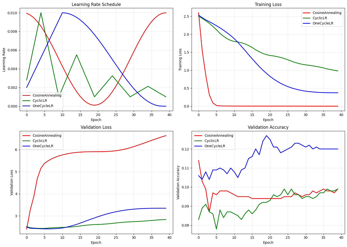
4.4 Comparing Advanced Schedulers#
# Compare advanced schedulers
plot_lr_schedules(
    [history_cosine, history_cyclic, history_onecycle],
    ['CosineAnnealing', 'CyclicLR', 'OneCycleLR'],
    colors=['red', 'green', 'blue']
)
5. Adaptive Scheduling with Warmup#
Let’s implement adaptive scheduling strategies including warmup and plateau-based reduction.
5.1 Warmup Scheduler#
# Create model with warmup scheduler
model_warmup = SimpleNet()

warmup_lr = braintools.optim.WarmupScheduler(
    base_lr=0.01,
    warmup_epochs=5,
    warmup_start_lr=0.0001,
)

optimizer_warmup = braintools.optim.Adam(lr=warmup_lr)

print("Training with Warmup + Exponential Decay...")
history_warmup = train_with_scheduler(
    model_warmup, optimizer_warmup,
    X_train, y_train, X_val, y_val,
    n_epochs=40, batch_size=128
)
Training with Warmup + Exponential Decay...
Epoch 10/40 - Loss: 0.0104, Acc: 0.9996, Val Loss: 6.5678, Val Acc: 0.1150, LR: 0.010000
Epoch 20/40 - Loss: 0.0008, Acc: 1.0000, Val Loss: 6.9188, Val Acc: 0.1160, LR: 0.010000
Epoch 30/40 - Loss: 0.0004, Acc: 1.0000, Val Loss: 7.1367, Val Acc: 0.1170, LR: 0.010000
Epoch 40/40 - Loss: 0.0002, Acc: 1.0000, Val Loss: 7.3129, Val Acc: 0.1170, LR: 0.010000
5.2 ReduceLROnPlateau Scheduler#
# Train with ReduceLROnPlateau
def train_with_plateau_scheduler(
    model, optimizer_class, X_train, y_train, X_val, y_val,
    n_epochs=50, batch_size=128
):
    """Special training loop for ReduceLROnPlateau."""

    plateau_lr = braintools.optim.ReduceLROnPlateau(
        base_lr=0.01,
        mode='min',
        factor=0.5,
        patience=5
    )

    optimizer = optimizer_class(lr=plateau_lr)

    # Get parameter states
    param_states = braintools.optim.UniqueStateManager(
        model.states(brainstate.ParamState)
    ).to_pytree()

    optimizer.register_trainable_weights(param_states)

    @brainstate.transform.jit
    def train_step(X_batch, y_batch):
        loss, grads, acc = compute_loss_and_grads(model, X_batch, y_batch, param_states)
        optimizer.update(grads)
        return loss, acc

    @brainstate.transform.jit
    def eval_step(X_batch, y_batch):
        loss, _, acc = compute_loss_and_grads(model, X_batch, y_batch, param_states)
        return loss, acc

    history = {
        'train_loss': [],
        'val_loss': [],
        'val_acc': [],
        'lr': []
    }

    n_batches = len(X_train) // batch_size

    for epoch in range(n_epochs):
        # Training
        perm = brainstate.random.permutation(len(X_train))
        X_train_shuffled = X_train[perm]
        y_train_shuffled = y_train[perm]

        train_losses = []
        for batch_idx in range(n_batches):
            start_idx = batch_idx * batch_size
            end_idx = start_idx + batch_size
            X_batch = X_train_shuffled[start_idx:end_idx]
            y_batch = y_train_shuffled[start_idx:end_idx]

            loss, _ = train_step(X_batch, y_batch)
            train_losses.append(float(loss))

        # Validation
        val_loss, val_acc = eval_step(X_val, y_val)
        val_loss = float(val_loss)

        # Update scheduler based on validation loss
        plateau_lr.step(metric=val_loss)

        # Record metrics
        history['train_loss'].append(np.mean(train_losses))
        history['val_loss'].append(val_loss)
        history['val_acc'].append(float(val_acc))
        history['lr'].append(plateau_lr.get_lr()[0])

        if (epoch + 1) % 10 == 0:
            print(f"Epoch {epoch + 1}/{n_epochs} - "
                  f"Train Loss: {history['train_loss'][-1]:.4f}, "
                  f"Val Loss: {val_loss:.4f}, "
                  f"LR: {plateau_lr.get_lr()[0]:.6f}")

    return history


# Create model for plateau scheduler
model_plateau = SimpleNet()

print("Training with ReduceLROnPlateau...")
history_plateau = train_with_plateau_scheduler(
    model_plateau, braintools.optim.Adam,
    X_train, y_train, X_val, y_val,
    n_epochs=40, batch_size=128
)
Training with ReduceLROnPlateau...
Epoch 10/40 - Train Loss: 0.0039, Val Loss: 5.7269, LR: 0.005000
Epoch 20/40 - Train Loss: 0.0019, Val Loss: 5.9691, LR: 0.001250
Epoch 30/40 - Train Loss: 0.0016, Val Loss: 6.0443, LR: 0.000625
Epoch 40/40 - Train Loss: 0.0015, Val Loss: 6.0727, LR: 0.000156
6. Scheduler Composition#
Let’s create composite schedulers that combine multiple scheduling strategies.
# Create a complex scheduler: warmup -> cosine -> exponential
warmup = braintools.optim.WarmupScheduler(
    base_lr=0.01, warmup_epochs=5, warmup_start_lr=0.0001,
)

cosine = braintools.optim.CosineAnnealingLR(
    base_lr=0.01, T_max=15, eta_min=0.001
)

exponential = braintools.optim.ExponentialLR(
    base_lr=0.001, gamma=0.9
)

chained_scheduler = braintools.optim.SequentialLR(
    schedulers=[warmup, cosine, exponential],
    milestones=[5, 20]  # Switch at epoch 5 and 20
)

# Train with chained scheduler
model_chained = SimpleNet()
optimizer_chained = braintools.optim.Adam(lr=chained_scheduler)

print("Training with Chained Scheduler (Warmup -> Cosine -> Exponential)...")
history_chained = train_with_scheduler(
    model_chained, optimizer_chained,
    X_train, y_train, X_val, y_val,
    n_epochs=40, batch_size=128
)
Training with Chained Scheduler (Warmup -> Cosine -> Exponential)...
Epoch 10/40 - Loss: 0.0030, Acc: 1.0000, Val Loss: 5.9528, Val Acc: 0.1060, LR: 0.003250
Epoch 20/40 - Loss: 0.0009, Acc: 1.0000, Val Loss: 6.4556, Val Acc: 0.1070, LR: 0.000122
Epoch 30/40 - Loss: 0.0004, Acc: 1.0000, Val Loss: 6.7822, Val Acc: 0.1060, LR: 0.000042
Epoch 40/40 - Loss: 0.0003, Acc: 1.0000, Val Loss: 7.0344, Val Acc: 0.1050, LR: 0.000015
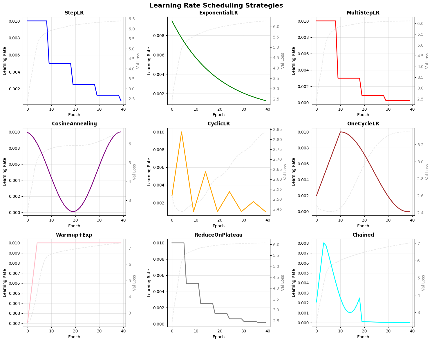
7. Visualizing Learning Rate Trajectories#
Let’s create comprehensive visualizations of all our learning rate scheduling strategies.
def visualize_all_schedules():
    """Create a comprehensive visualization of all LR schedules."""

    fig, axes = plt.subplots(3, 3, figsize=(15, 12))

    schedules_data = [
        (history_step, 'StepLR', 'blue'),
        (history_exp, 'ExponentialLR', 'green'),
        (history_multistep, 'MultiStepLR', 'red'),
        (history_cosine, 'CosineAnnealing', 'purple'),
        (history_cyclic, 'CyclicLR', 'orange'),
        (history_onecycle, 'OneCycleLR', 'brown'),
        (history_warmup, 'Warmup+Exp', 'pink'),
        (history_plateau, 'ReduceOnPlateau', 'gray'),
        (history_chained, 'Chained', 'cyan')
    ]

    for idx, (history, name, color) in enumerate(schedules_data):
        ax = axes[idx // 3, idx % 3]

        # Plot learning rate
        ax.plot(history['lr'], color=color, linewidth=2)
        ax.set_title(name, fontsize=12, fontweight='bold')
        ax.set_xlabel('Epoch')
        ax.set_ylabel('Learning Rate')
        ax.grid(True, alpha=0.3)

        # Add validation loss on secondary y-axis
        ax2 = ax.twinx()
        ax2.plot(history['val_loss'], color='lightgray', alpha=0.5, linestyle='--')
        ax2.set_ylabel('Val Loss', color='gray')
        ax2.tick_params(axis='y', labelcolor='gray')

    plt.suptitle('Learning Rate Scheduling Strategies', fontsize=16, fontweight='bold')
    plt.tight_layout()
    plt.show()


visualize_all_schedules()
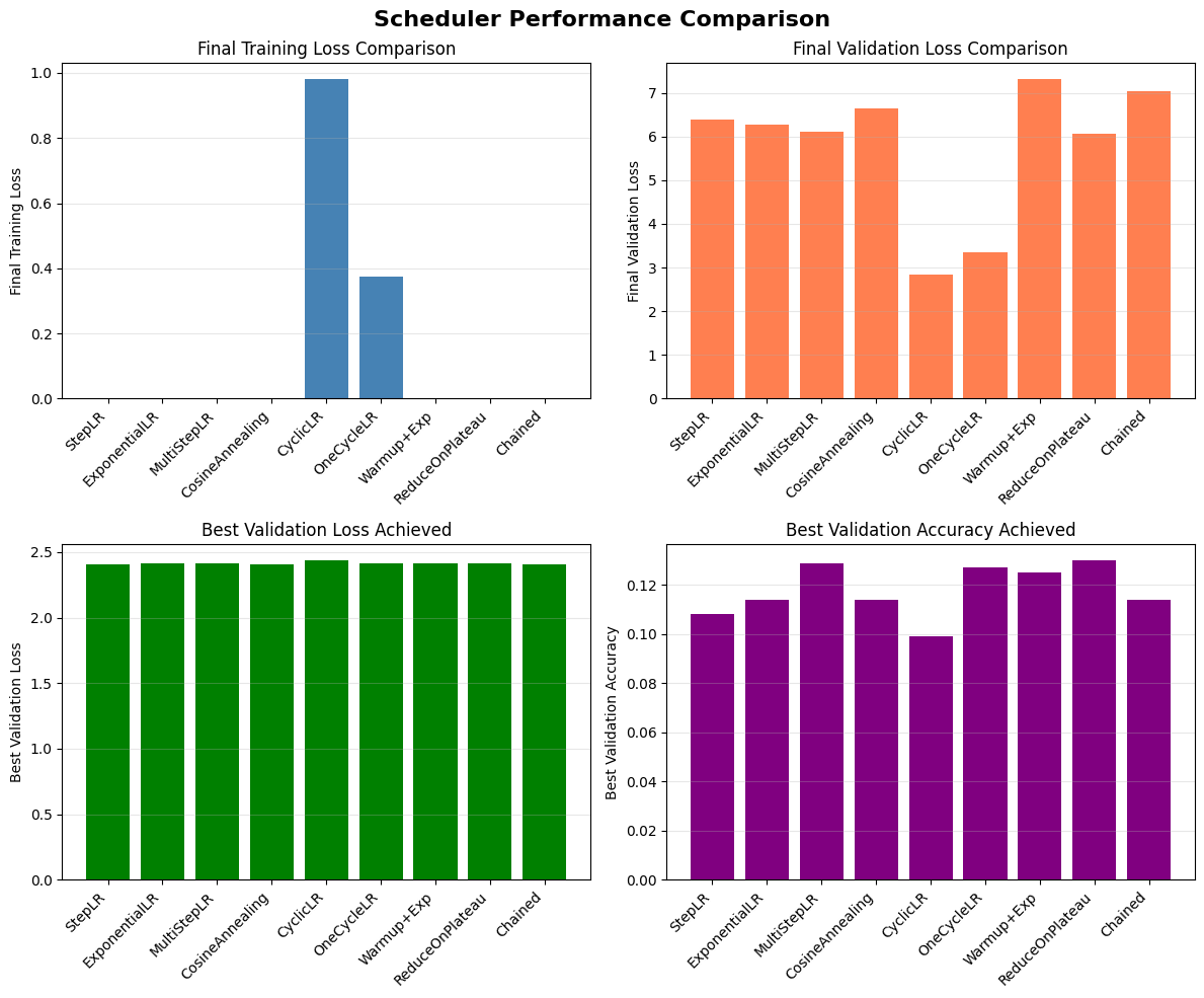
8. Performance Comparison#
Let’s compare the final performance of all scheduling strategies.
def compare_scheduler_performance():
    """Compare final metrics for all schedulers."""

    schedulers = [
        'StepLR', 'ExponentialLR', 'MultiStepLR',
        'CosineAnnealing', 'CyclicLR', 'OneCycleLR',
        'Warmup+Exp', 'ReduceOnPlateau', 'Chained'
    ]

    histories = [
        history_step, history_exp, history_multistep,
        history_cosine, history_cyclic, history_onecycle,
        history_warmup, history_plateau, history_chained
    ]

    # Collect metrics
    final_train_loss = [h['train_loss'][-1] for h in histories]
    final_val_loss = [h['val_loss'][-1] for h in histories]
    best_val_loss = [min(h['val_loss']) for h in histories]
    best_val_acc = [max(h.get('val_acc', [0])) for h in histories]

    # Create comparison plot
    fig, axes = plt.subplots(2, 2, figsize=(12, 10))

    # Final training loss
    ax = axes[0, 0]
    bars = ax.bar(range(len(schedulers)), final_train_loss, color='steelblue')
    ax.set_xticks(range(len(schedulers)))
    ax.set_xticklabels(schedulers, rotation=45, ha='right')
    ax.set_ylabel('Final Training Loss')
    ax.set_title('Final Training Loss Comparison')
    ax.grid(True, alpha=0.3, axis='y')

    # Final validation loss
    ax = axes[0, 1]
    bars = ax.bar(range(len(schedulers)), final_val_loss, color='coral')
    ax.set_xticks(range(len(schedulers)))
    ax.set_xticklabels(schedulers, rotation=45, ha='right')
    ax.set_ylabel('Final Validation Loss')
    ax.set_title('Final Validation Loss Comparison')
    ax.grid(True, alpha=0.3, axis='y')

    # Best validation loss
    ax = axes[1, 0]
    bars = ax.bar(range(len(schedulers)), best_val_loss, color='green')
    ax.set_xticks(range(len(schedulers)))
    ax.set_xticklabels(schedulers, rotation=45, ha='right')
    ax.set_ylabel('Best Validation Loss')
    ax.set_title('Best Validation Loss Achieved')
    ax.grid(True, alpha=0.3, axis='y')

    # Best validation accuracy
    ax = axes[1, 1]
    bars = ax.bar(range(len(schedulers)), best_val_acc, color='purple')
    ax.set_xticks(range(len(schedulers)))
    ax.set_xticklabels(schedulers, rotation=45, ha='right')
    ax.set_ylabel('Best Validation Accuracy')
    ax.set_title('Best Validation Accuracy Achieved')
    ax.grid(True, alpha=0.3, axis='y')

    plt.suptitle('Scheduler Performance Comparison', fontsize=16, fontweight='bold')
    plt.tight_layout()
    plt.show()

    # Print summary table
    print("\n" + "=" * 80)
    print(f"{'Scheduler':<20} {'Final Train Loss':<18} {'Best Val Loss':<18} {'Best Val Acc':<15}")
    print("=" * 80)

    for name, ftl, bvl, bva in zip(schedulers, final_train_loss, best_val_loss, best_val_acc):
        print(f"{name:<20} {ftl:<18.4f} {bvl:<18.4f} {bva:<15.4f}")
    print("=" * 80)


compare_scheduler_performance()
================================================================================
Scheduler            Final Train Loss   Best Val Loss      Best Val Acc
================================================================================
StepLR               0.0008             2.4039             0.1080
ExponentialLR        0.0009             2.4179             0.1140
MultiStepLR          0.0013             2.4179             0.1290
CosineAnnealing      0.0006             2.4058             0.1140
CyclicLR             0.9810             2.4366             0.0990
OneCycleLR           0.3730             2.4134             0.1270
Warmup+Exp           0.0002             2.4117             0.1250
ReduceOnPlateau      0.0015             2.4152             0.1300
Chained              0.0003             2.4091             0.1140
================================================================================
Summary and Best Practices#
Key Takeaways#
Basic Schedulers (StepLR, ExponentialLR, MultiStepLR)
Simple and predictable
Good for well-understood problems
StepLR: Discrete drops at fixed intervals
ExponentialLR: Smooth exponential decay
MultiStepLR: Custom control over decay points
Advanced Schedulers
CosineAnnealing: Smooth periodic decay, good for avoiding local minima
CyclicLR: Oscillating learning rates can help escape saddle points
OneCycleLR: Super-convergence for faster training
Adaptive Strategies
Warmup: Essential for large models and batch sizes
ReduceLROnPlateau: Automatically adapts to training progress
Chained Schedulers: Combine multiple strategies for complex training regimes
When to Use Each Scheduler#
Scheduler |
Best For |
Key Advantage |
|---|---|---|
StepLR |
Known training duration |
Simple and predictable |
ExponentialLR |
Smooth decay needed |
Gradual reduction |
MultiStepLR |
Domain-specific knowledge |
Precise control |
CosineAnnealing |
Avoiding local minima |
Smooth annealing |
CyclicLR |
Escaping saddle points |
Dynamic exploration |
OneCycleLR |
Fast convergence |
Super-convergence |
Warmup |
Large models/batches |
Stable initialization |
ReduceLROnPlateau |
Unknown optimal schedule |
Automatic adaptation |
Chained |
Complex training |
Maximum flexibility |
Exercises#
Custom Scheduler: Implement a polynomial decay scheduler where
lr = init_lr * (1 - epoch/max_epoch)^powerWarmup Variants: Create a cosine warmup instead of linear warmup
Adaptive Cyclic: Combine CyclicLR with ReduceLROnPlateau for adaptive cycling
Restart Strategies: Implement SGDR (SGD with warm restarts) using cosine annealing
Learning Rate Finder: Implement the learning rate range test to find optimal learning rates
Schedule Visualization: Create an interactive tool to visualize and compare different schedules before training