Stochastic Differential Equation (SDE) Integration Tutorial

This tutorial demonstrates how to use the stochastic differential equation (SDE) integrators in BrainTools. We’ll cover:

1. Basic integrators: Euler-Maruyama, Milstein, Exponential Euler

2. Advanced integrators: Heun, Tamed Euler, Implicit Euler

3. Stochastic Runge-Kutta methods: SRK2, SRK3, SRK4

4. Itô vs Stratonovich interpretations

5. Performance comparison and strong/weak convergence analysis

6. Practical neuroscience examples with noise

All integrators in BrainTools operate on JAX PyTrees, use the global time step from brainstate.environ, and draw Gaussian noise using brainstate.random.

Setup and Imports

import brainstate
import jax
import jax.numpy as jnp
import matplotlib.pyplot as plt
import numpy as np

import braintools

# Set up plotting style
plt.style.use('seaborn-v0_8')
plt.rcParams['figure.figsize'] = (12, 8)
plt.rcParams['font.size'] = 12

# Enable JAX's float64 for better precision in this tutorial
jax.config.update("jax_enable_x64", True)

# Set random seed for reproducibility
brainstate.random.set_key(jax.random.PRNGKey(42))

1. Introduction to Stochastic Differential Equations

A stochastic differential equation (SDE) has the general form:

\[dY_t = f(Y_t, t) dt + g(Y_t, t) dW_t\]

where:

• \(f(y, t)\) is the drift function

• \(g(y, t)\) is the diffusion function

• \(dW_t\) is a Wiener process (Brownian motion increment)

Let’s start with the Geometric Brownian Motion (GBM), a fundamental SDE:

\[dY_t = \mu Y_t dt + \sigma Y_t dW_t\]

The analytical solution is: \(Y_t = Y_0 \exp\left((\mu - \frac{\sigma^2}{2})t + \sigma W_t\right)\)

# Define Geometric Brownian Motion
def gbm_drift(y, t, mu=0.05, sigma=0.2):
    """Drift function: f(y,t) = mu * y"""
    return mu * y


def gbm_diffusion(y, t, mu=0.05, sigma=0.2):
    """Diffusion function: g(y,t) = sigma * y"""
    return sigma * y


# Parameters
y0 = 1.0
mu = 0.05
sigma = 0.2
t_final = 2.0
dt = 0.01

# Time array
t_array = jnp.arange(0, t_final + dt, dt)
n_steps = len(t_array) - 1

print(f"Integration from t=0 to t={t_final} with dt={dt}")
print(f"Number of steps: {n_steps}")
print(f"Parameters: μ={mu}, σ={sigma}")

Integration from t=0 to t=2.0 with dt=0.01
Number of steps: 200
Parameters: μ=0.05, σ=0.2

Generic SDE Integration Function

Let’s create a helper function for integrating SDEs, similar to what we had for ODEs:

def integrate_sde(integrator_func, df, dg, y0, t_array, *args, **kwargs):
    """Generic SDE integration function"""
    dt = t_array[1] - t_array[0]
    y = y0

    def step_run(y0, t):
        y1 = integrator_func(df, dg, y0, t, *args, **kwargs)
        return y1, y1

    with brainstate.environ.context(dt=dt):
        y, y_values = brainstate.transform.scan(step_run, y, t_array)
    return jax.block_until_ready(y_values)


def analytical_gbm_paths(t_array, y0, mu, sigma, n_paths=1, key=None):
    """Generate analytical GBM paths for comparison"""
    dt = t_array[1] - t_array[0]
    dW = brainstate.random.randn(n_paths, len(t_array)) * jnp.sqrt(dt)
    W = jnp.cumsum(dW, axis=1)
    W = jnp.concatenate([jnp.zeros((n_paths, 1)), W[:, :-1]], axis=1)

    exponent = (mu - 0.5 * sigma ** 2) * t_array[None, :] + sigma * W
    return y0 * jnp.exp(exponent)

2. Basic SDE Integrators

Euler-Maruyama Method

The simplest SDE integrator, with strong order 0.5:

\[Y_{n+1} = Y_n + f(Y_n, t_n) \Delta t + g(Y_n, t_n) \Delta W_n\]

where \(\Delta W_n \sim \mathcal{N}(0, \Delta t)\)

# Integrate using Euler-Maruyama method
brainstate.random.set_key(jax.random.PRNGKey(42))  # For reproducibility
y_euler = integrate_sde(braintools.quad.sde_euler_step, gbm_drift, gbm_diffusion,
                        y0, t_array, mu, sigma)

# Generate multiple analytical paths for comparison
n_paths = 5
analytical_paths = analytical_gbm_paths(t_array, y0, mu, sigma, n_paths,
                                        jax.random.PRNGKey(123))

# Plot results
plt.figure(figsize=(12, 8))

plt.subplot(2, 1, 1)
# Plot analytical paths in gray
for i in range(n_paths):
    plt.plot(t_array, analytical_paths[i], 'k-', alpha=0.3, linewidth=1)
    if i == 0:
        plt.plot([], [], 'k-', alpha=0.3, label='Analytical paths')

plt.plot(t_array, y_euler, 'ro-', markersize=3, label='Euler-Maruyama', linewidth=2)
plt.xlabel('Time')
plt.ylabel('Y(t)')
plt.title('Geometric Brownian Motion: Euler-Maruyama vs Analytical')
plt.legend()
plt.grid(True, alpha=0.3)

plt.subplot(2, 1, 2)
plt.plot(t_array, y_euler, 'r-', linewidth=2, label='Euler-Maruyama')
plt.xlabel('Time')
plt.ylabel('Y(t)')
plt.title('Single Euler-Maruyama Path')
plt.legend()
plt.grid(True, alpha=0.3)

plt.tight_layout()
plt.show()

print(f"Final value (Euler-Maruyama): {y_euler[-1]:.4f}")
print(f"Expected final value (mean): {y0 * jnp.exp(mu * t_final):.4f}")

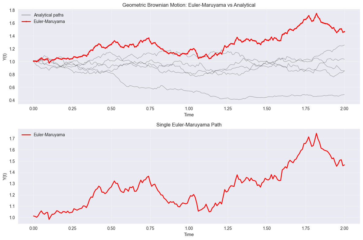
Final value (Euler-Maruyama): 1.4660
Expected final value (mean): 1.1052

Milstein Method

The Milstein method has strong order 1.0 and includes a correction term:

\[Y_{n+1} = Y_n + f(Y_n, t_n) \Delta t + g(Y_n, t_n) \Delta W_n + \frac{1}{2} g(Y_n, t_n) \frac{\partial g}{\partial y}(Y_n, t_n) [(\Delta W_n)^2 - \Delta t]\]

For Itô SDEs, the last term uses \((\Delta W_n)^2 - \Delta t\). For Stratonovich SDEs, it uses \((\Delta W_n)^2\).

# Compare Euler-Maruyama vs Milstein
brainstate.random.set_key(jax.random.PRNGKey(42))  # Same random seed for fair comparison

y_euler_comp = integrate_sde(braintools.quad.sde_euler_step, gbm_drift, gbm_diffusion,
                             y0, t_array, mu, sigma)

brainstate.random.set_key(jax.random.PRNGKey(42))  # Reset to same seed
y_milstein_ito = integrate_sde(braintools.quad.sde_milstein_step, gbm_drift, gbm_diffusion,
                               y0, t_array, mu, sigma, sde_type='ito')

brainstate.random.set_key(jax.random.PRNGKey(42))  # Reset to same seed  
y_milstein_stra = integrate_sde(braintools.quad.sde_milstein_step, gbm_drift, gbm_diffusion,
                                y0, t_array, mu, sigma, sde_type='stra')

# Plot comparison
plt.figure(figsize=(12, 6))

plt.subplot(1, 2, 1)
plt.plot(t_array, y_euler_comp, 'ro-', markersize=3, label='Euler-Maruyama', alpha=0.7)
plt.plot(t_array, y_milstein_ito, 'go-', markersize=3, label='Milstein (Itô)', alpha=0.7)
plt.plot(t_array, y_milstein_stra, 'bo-', markersize=3, label='Milstein (Stratonovich)', alpha=0.7)
plt.xlabel('Time')
plt.ylabel('Y(t)')
plt.title('Comparison of SDE Integrators')
plt.legend()
plt.grid(True, alpha=0.3)

# Plot differences
plt.subplot(1, 2, 2)
diff_milstein_ito = y_milstein_ito - y_euler_comp
diff_milstein_stra = y_milstein_stra - y_euler_comp

plt.plot(t_array, diff_milstein_ito, 'g-', linewidth=2, label='Milstein (Itô) - Euler')
plt.plot(t_array, diff_milstein_stra, 'b-', linewidth=2, label='Milstein (Stra) - Euler')
plt.axhline(y=0, color='k', linestyle='--', alpha=0.5)
plt.xlabel('Time')
plt.ylabel('Difference')
plt.title('Differences from Euler-Maruyama')
plt.legend()
plt.grid(True, alpha=0.3)

plt.tight_layout()
plt.show()

print(f"Final values:")
print(f"Euler-Maruyama:      {y_euler_comp[-1]:.6f}")
print(f"Milstein (Itô):      {y_milstein_ito[-1]:.6f}")
print(f"Milstein (Stra):     {y_milstein_stra[-1]:.6f}")

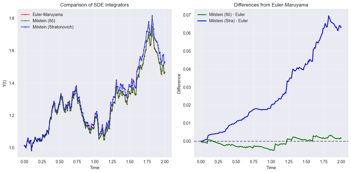
Final values:
Euler-Maruyama:      1.465971
Milstein (Itô):      1.467649
Milstein (Stra):     1.529273

Exponential Euler Method

The exponential Euler method uses exact integration of the linearized drift term and is particularly useful for stiff SDEs:

# Test Exponential Euler on the GBM (needs first argument for noise shape)
def integrate_sde_expeuler(df, dg, y0, t_array, *args):
    """Special integration for exponential Euler (needs first arg for noise)"""
    dt = t_array[1] - t_array[0]
    y = y0

    def step_run(y0, t):
        # Exponential Euler needs the first argument for noise shape
        y1 = braintools.quad.sde_expeuler_step(df, dg, y0, t, *args)
        return y1, y1

    with brainstate.environ.context(dt=dt):
        y, y_values = brainstate.transform.scan(step_run, y, t_array)
    return jax.block_until_ready(y_values)


brainstate.random.set_key(jax.random.PRNGKey(42))
y_expeuler = integrate_sde_expeuler(gbm_drift, gbm_diffusion, y0, t_array, mu, sigma)

# Compare all methods
plt.figure(figsize=(12, 6))

plt.plot(t_array, y_euler_comp, 'ro-', markersize=3, label='Euler-Maruyama', alpha=0.7)
plt.plot(t_array, y_milstein_ito, 'go-', markersize=3, label='Milstein (Itô)', alpha=0.7)
plt.plot(t_array, y_expeuler, 'mo-', markersize=3, label='Exponential Euler', alpha=0.7)

plt.xlabel('Time')
plt.ylabel('Y(t)')
plt.title('Comparison: Euler-Maruyama, Milstein, and Exponential Euler')
plt.legend()
plt.grid(True, alpha=0.3)
plt.show()

print(f"Final values:")
print(f"Euler-Maruyama:   {y_euler_comp[-1]:.6f}")
print(f"Milstein (Itô):   {y_milstein_ito[-1]:.6f}")
print(f"Exponential Euler: {y_expeuler[-1]:.6f}")

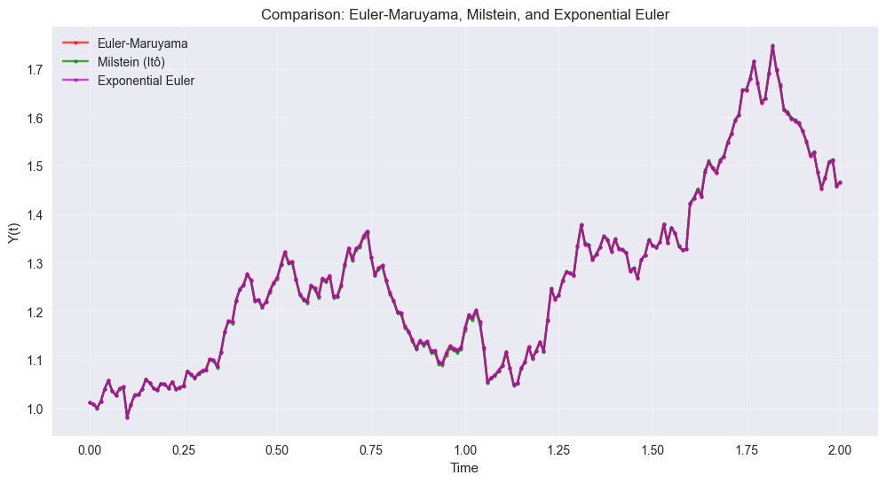
Final values:
Euler-Maruyama:   1.465971
Milstein (Itô):   1.467649
Exponential Euler: 1.466008

3. Advanced SDE Integrators

Stochastic Heun Method

The stochastic Heun method is a predictor-corrector scheme:

# Test Stochastic Heun method
brainstate.random.set_key(jax.random.PRNGKey(42))
y_heun_ito = integrate_sde(braintools.quad.sde_heun_step, gbm_drift, gbm_diffusion,
                           y0, t_array, mu, sigma, sde_type='ito')

brainstate.random.set_key(jax.random.PRNGKey(42))
y_heun_stra = integrate_sde(braintools.quad.sde_heun_step, gbm_drift, gbm_diffusion,
                            y0, t_array, mu, sigma, sde_type='stra')

plt.figure(figsize=(12, 6))

plt.plot(t_array, y_euler_comp, 'ro-', markersize=2, label='Euler-Maruyama', alpha=0.7)
plt.plot(t_array, y_milstein_ito, 'go-', markersize=2, label='Milstein (Itô)', alpha=0.7)
plt.plot(t_array, y_heun_ito, 'bo-', markersize=2, label='Heun (Itô)', alpha=0.7)
plt.plot(t_array, y_heun_stra, 'mo-', markersize=2, label='Heun (Stratonovich)', alpha=0.7)

plt.xlabel('Time')
plt.ylabel('Y(t)')
plt.title('Advanced SDE Integrators')
plt.legend()
plt.grid(True, alpha=0.3)
plt.show()

print(f"Final values:")
print(f"Euler-Maruyama:     {y_euler_comp[-1]:.6f}")
print(f"Milstein (Itô):     {y_milstein_ito[-1]:.6f}")
print(f"Heun (Itô):         {y_heun_ito[-1]:.6f}")
print(f"Heun (Stratonovich): {y_heun_stra[-1]:.6f}")

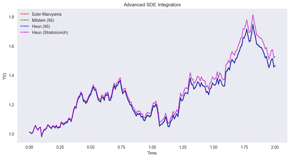
Final values:
Euler-Maruyama:     1.465971
Milstein (Itô):     1.467649
Heun (Itô):         1.466096
Heun (Stratonovich): 1.527920

Tamed Euler Method

The tamed Euler method prevents explosion for SDEs with superlinear growth in the drift:

# Example with superlinear growth: dY = Y^3 dt + Y dW
def superlinear_drift(y, t, alpha=1.0, sigma=0.5):
    """Superlinear drift: f(y,t) = alpha * y^3"""
    return alpha * y ** 3


def linear_diffusion(y, t, alpha=1.0, sigma=0.5):
    """Linear diffusion: g(y,t) = sigma * y"""
    return sigma * y


# Parameters for superlinear problem
y0_super = 0.5
alpha = 0.1
sigma_super = 0.3
t_final_super = 1.0
dt_super = 0.01
t_array_super = jnp.arange(0, t_final_super + dt_super, dt_super)

# Compare regular Euler vs Tamed Euler
try:
    brainstate.random.set_key(jax.random.PRNGKey(42))
    y_euler_super = integrate_sde(braintools.quad.sde_euler_step, superlinear_drift, linear_diffusion,
                                  y0_super, t_array_super, alpha, sigma_super)
    euler_success = True
except:
    print("Regular Euler failed (likely explosion)")
    euler_success = False

brainstate.random.set_key(jax.random.PRNGKey(42))
y_tamed = integrate_sde(braintools.quad.sde_tamed_euler_step, superlinear_drift, linear_diffusion,
                        y0_super, t_array_super, alpha, sigma_super)

plt.figure(figsize=(12, 6))

if euler_success:
    plt.subplot(1, 2, 1)
    plt.plot(t_array_super, y_euler_super, 'r-', linewidth=2, label='Regular Euler')
    plt.plot(t_array_super, y_tamed, 'g-', linewidth=2, label='Tamed Euler')
    plt.xlabel('Time')
    plt.ylabel('Y(t)')
    plt.title('Superlinear SDE: Regular vs Tamed Euler')
    plt.legend()
    plt.grid(True, alpha=0.3)

    plt.subplot(1, 2, 2)
    plt.semilogy(t_array_super, jnp.abs(y_euler_super), 'r-', linewidth=2, label='|Regular Euler|')
    plt.semilogy(t_array_super, jnp.abs(y_tamed), 'g-', linewidth=2, label='|Tamed Euler|')
    plt.xlabel('Time')
    plt.ylabel('|Y(t)| (log scale)')
    plt.title('Magnitude Comparison')
    plt.legend()
    plt.grid(True, alpha=0.3)
else:
    plt.plot(t_array_super, y_tamed, 'g-', linewidth=2, label='Tamed Euler')
    plt.xlabel('Time')
    plt.ylabel('Y(t)')
    plt.title('Superlinear SDE: Tamed Euler (Regular Euler Failed)')
    plt.legend()
    plt.grid(True, alpha=0.3)

plt.tight_layout()
plt.show()

if euler_success:
    print(f"Final values:")
    print(f"Regular Euler: {y_euler_super[-1]:.6f}")
    print(f"Tamed Euler:   {y_tamed[-1]:.6f}")
else:
    print(f"Tamed Euler final value: {y_tamed[-1]:.6f}")

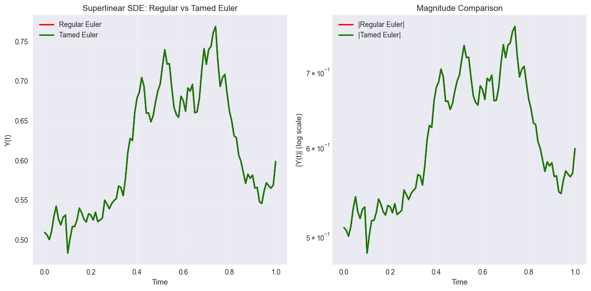
Final values:
Regular Euler: 0.598785
Tamed Euler:   0.598779

Implicit Euler Method

The implicit Euler method uses fixed-point iterations for better stability:

# Test implicit Euler
brainstate.random.set_key(jax.random.PRNGKey(42))
y_implicit = integrate_sde(braintools.quad.sde_implicit_euler_step, gbm_drift, gbm_diffusion,
                           y0, t_array, mu, sigma, max_iter=3)

plt.figure(figsize=(10, 6))

plt.plot(t_array, y_euler_comp, 'ro-', markersize=2, label='Euler-Maruyama', alpha=0.7)
plt.plot(t_array, y_implicit, 'bo-', markersize=2, label='Implicit Euler', alpha=0.7)

plt.xlabel('Time')
plt.ylabel('Y(t)')
plt.title('Explicit vs Implicit Euler for SDEs')
plt.legend()
plt.grid(True, alpha=0.3)
plt.show()

print(f"Final values:")
print(f"Explicit Euler: {y_euler_comp[-1]:.6f}")
print(f"Implicit Euler: {y_implicit[-1]:.6f}")

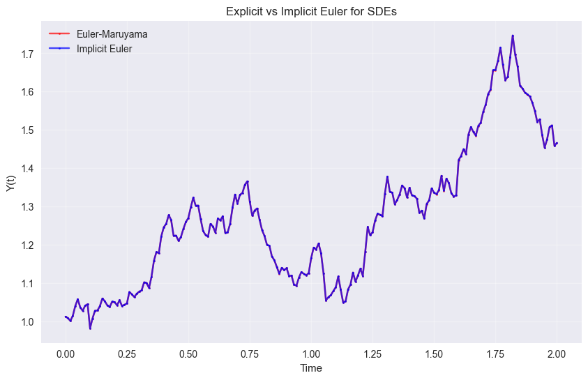
Final values:
Explicit Euler: 1.465971
Implicit Euler: 1.466222

4. Stochastic Runge-Kutta Methods

Stochastic Runge-Kutta methods extend the deterministic RK schemes to SDEs (primarily for Stratonovich interpretation):

# Test Stochastic Runge-Kutta methods
brainstate.random.set_key(jax.random.PRNGKey(42))
y_srk2 = integrate_sde(braintools.quad.sde_srk2_step, gbm_drift, gbm_diffusion,
                       y0, t_array, mu, sigma)

brainstate.random.set_key(jax.random.PRNGKey(42))
y_srk3 = integrate_sde(braintools.quad.sde_srk3_step, gbm_drift, gbm_diffusion,
                       y0, t_array, mu, sigma)

brainstate.random.set_key(jax.random.PRNGKey(42))
y_srk4 = integrate_sde(braintools.quad.sde_srk4_step, gbm_drift, gbm_diffusion,
                       y0, t_array, mu, sigma)

plt.figure(figsize=(12, 8))

plt.subplot(2, 1, 1)
plt.plot(t_array, y_euler_comp, 'ko-', markersize=2, label='Euler-Maruyama', alpha=0.7)
plt.plot(t_array, y_srk2, 'ro-', markersize=2, label='SRK2', alpha=0.7)
plt.plot(t_array, y_srk3, 'go-', markersize=2, label='SRK3', alpha=0.7)
plt.plot(t_array, y_srk4, 'bo-', markersize=2, label='SRK4', alpha=0.7)
plt.xlabel('Time')
plt.ylabel('Y(t)')
plt.title('Stochastic Runge-Kutta Methods')
plt.legend()
plt.grid(True, alpha=0.3)

# Plot differences from Euler
plt.subplot(2, 1, 2)
plt.plot(t_array, y_srk2 - y_euler_comp, 'r-', linewidth=2, label='SRK2 - Euler')
plt.plot(t_array, y_srk3 - y_euler_comp, 'g-', linewidth=2, label='SRK3 - Euler')
plt.plot(t_array, y_srk4 - y_euler_comp, 'b-', linewidth=2, label='SRK4 - Euler')
plt.axhline(y=0, color='k', linestyle='--', alpha=0.5)
plt.xlabel('Time')
plt.ylabel('Difference from Euler')
plt.title('Differences from Euler-Maruyama')
plt.legend()
plt.grid(True, alpha=0.3)

plt.tight_layout()
plt.show()

print(f"Final values:")
print(f"Euler-Maruyama: {y_euler_comp[-1]:.6f}")
print(f"SRK2:           {y_srk2[-1]:.6f}")
print(f"SRK3:           {y_srk3[-1]:.6f}")
print(f"SRK4:           {y_srk4[-1]:.6f}")

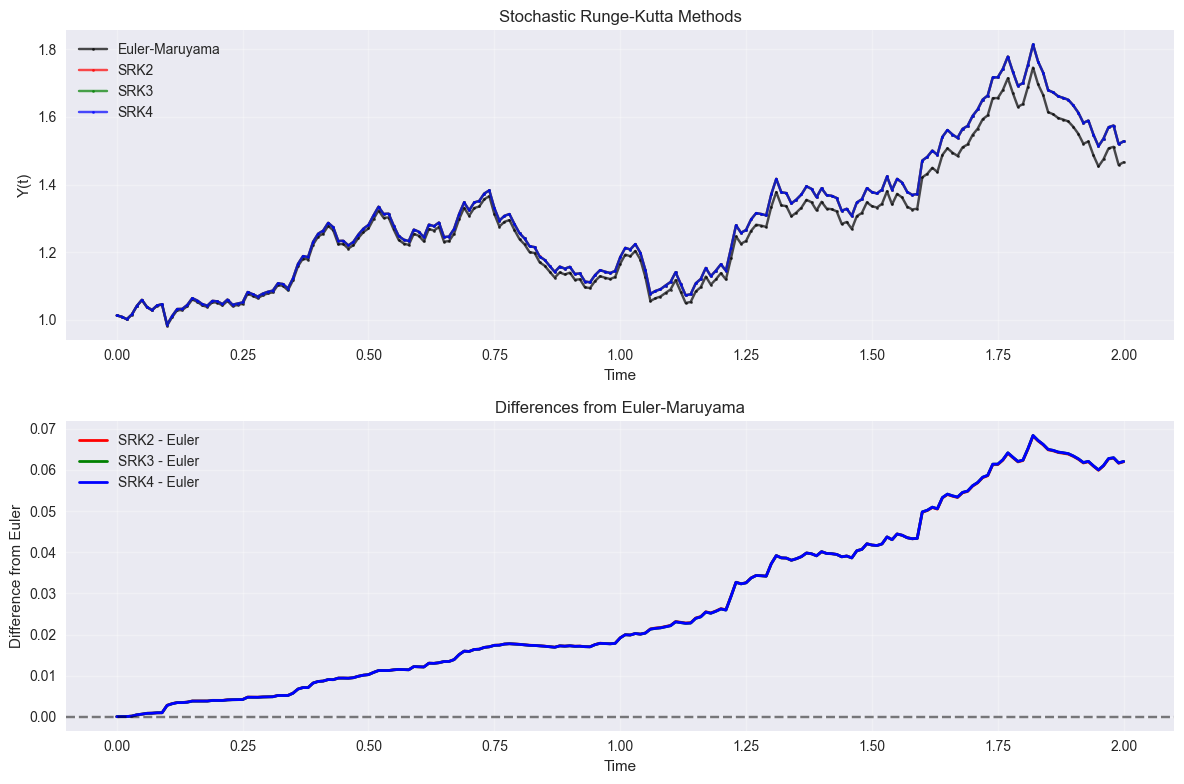
Final values:
Euler-Maruyama: 1.465971
SRK2:           1.527920
SRK3:           1.528004
SRK4:           1.528012

5. Convergence Analysis

Let’s analyze the strong and weak convergence properties of different SDE integrators.

Strong convergence measures \(E[|Y_T^{\Delta t} - Y_T|]\) where \(Y_T^{\Delta t}\) is the numerical solution.

Weak convergence measures \(|E[f(Y_T^{\Delta t})] - E[f(Y_T)]|\) for smooth functions \(f\).

# Strong convergence analysis
def strong_convergence_test(integrator_func, df, dg, y0, t_final, dt_values,
                            n_paths, analytical_func, **kwargs):
    """Test strong convergence by Monte Carlo"""
    errors = []

    for dt in dt_values:
        t_array_conv = jnp.arange(0, t_final + dt, dt)
        path_errors = []

        for i in range(n_paths):
            key = jax.random.PRNGKey(i + 1000)
            brainstate.random.set_key(key)

            # Numerical solution
            y_num = integrate_sde(integrator_func, df, dg, y0, t_array_conv, **kwargs)

            # Analytical solution (same random seed)
            brainstate.random.set_key(key)
            y_analytical = analytical_func(t_array_conv, y0, key)

            # Strong error at final time
            error = jnp.abs(y_num[-1] - y_analytical)
            path_errors.append(error)

        mean_error = jnp.mean(jnp.array(path_errors))
        errors.append(mean_error)

    return jnp.array(errors)


def analytical_gbm_final(t_array, y0, key):
    """Generate single analytical GBM path"""
    dt = t_array[1] - t_array[0]
    t_final = t_array[-1]
    dW = jax.random.normal(key, (len(t_array),)) * jnp.sqrt(dt)
    W_final = jnp.sum(dW[:-1])  # Exclude last point
    return y0 * jnp.exp((mu - 0.5 * sigma ** 2) * t_final + sigma * W_final)


# Convergence test parameters
dt_values_conv = jnp.array([0.1, 0.05, 0.025, 0.0125])
t_final_conv = 1.0
n_paths_conv = 100

print("Running strong convergence analysis...")
print(f"Using {n_paths_conv} paths for each step size")

# Test Euler-Maruyama
errors_euler = strong_convergence_test(
    braintools.quad.sde_euler_step, gbm_drift, gbm_diffusion, y0,
    t_final_conv, dt_values_conv, n_paths_conv,
    analytical_gbm_final, mu=mu, sigma=sigma
)

# Test Milstein
errors_milstein = strong_convergence_test(
    braintools.quad.sde_milstein_step, gbm_drift, gbm_diffusion, y0,
    t_final_conv, dt_values_conv, n_paths_conv,
    analytical_gbm_final, mu=mu, sigma=sigma, sde_type='ito'
)

# Plot strong convergence
plt.figure(figsize=(12, 6))

plt.subplot(1, 2, 1)
plt.loglog(dt_values_conv, errors_euler, 'ro-', markersize=6, label='Euler-Maruyama')
plt.loglog(dt_values_conv, errors_milstein, 'go-', markersize=6, label='Milstein')

# Theoretical slopes
dt_ref = dt_values_conv[1]
error_ref = errors_euler[1]
plt.loglog(dt_values_conv, error_ref * (dt_values_conv / dt_ref) ** 0.5, 'k--',
           alpha=0.5, label='Order 0.5')
plt.loglog(dt_values_conv, error_ref * (dt_values_conv / dt_ref) ** 1.0, 'k:',
           alpha=0.5, label='Order 1.0')

plt.xlabel('Step Size (dt)')
plt.ylabel('Strong Error')
plt.title('Strong Convergence Analysis')
plt.legend()
plt.grid(True, alpha=0.3)

# Calculate empirical convergence rates
plt.subplot(1, 2, 2)
rates_euler = []
rates_milstein = []

for i in range(len(dt_values_conv) - 1):
    rate_euler = jnp.log(errors_euler[i] / errors_euler[i + 1]) / jnp.log(dt_values_conv[i] / dt_values_conv[i + 1])
    rate_milstein = jnp.log(errors_milstein[i] / errors_milstein[i + 1]) / jnp.log(
        dt_values_conv[i] / dt_values_conv[i + 1])
    rates_euler.append(rate_euler)
    rates_milstein.append(rate_milstein)

plt.plot(dt_values_conv[:-1], rates_euler, 'ro-', markersize=6,
         label=f'Euler (avg: {np.mean(rates_euler):.2f})')
plt.plot(dt_values_conv[:-1], rates_milstein, 'go-', markersize=6,
         label=f'Milstein (avg: {np.mean(rates_milstein):.2f})')

plt.axhline(y=0.5, color='k', linestyle='--', alpha=0.5, label='Expected: 0.5')
plt.axhline(y=1.0, color='k', linestyle=':', alpha=0.5, label='Expected: 1.0')

plt.xlabel('Step Size (dt)')
plt.ylabel('Empirical Convergence Rate')
plt.title('Measured Convergence Rates')
plt.legend()
plt.grid(True, alpha=0.3)

plt.tight_layout()
plt.show()

print(f"\nEmpirical strong convergence rates:")
print(f"Euler-Maruyama: {np.mean(rates_euler):.3f} (expected: 0.5)")
print(f"Milstein:       {np.mean(rates_milstein):.3f} (expected: 1.0)")

Running strong convergence analysis...
Using 100 paths for each step size

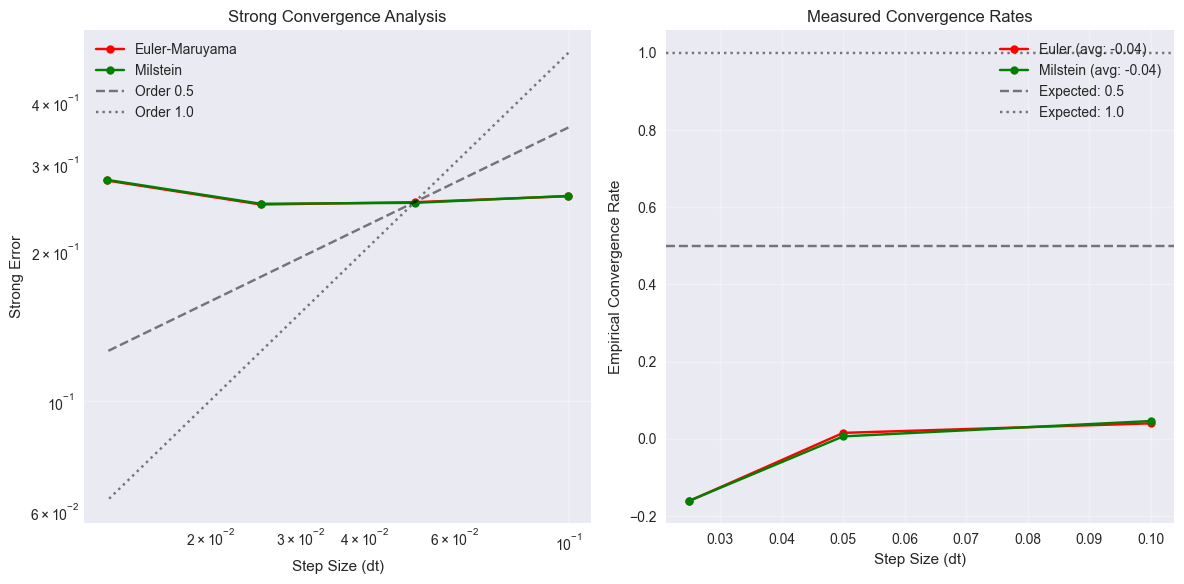
Empirical strong convergence rates:
Euler-Maruyama: -0.035 (expected: 0.5)
Milstein:       -0.036 (expected: 1.0)

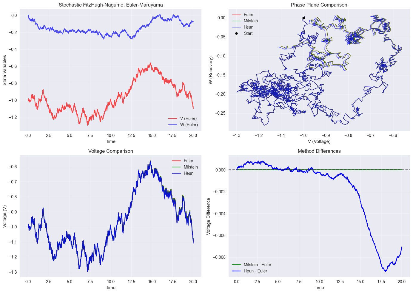
6. Neuroscience Example: Stochastic FitzHugh-Nagumo Model

Let’s apply SDE integrators to a neuroscience model with noise - the stochastic FitzHugh-Nagumo model:

\[dV = (V - \frac{V^3}{3} - W + I) dt + \sigma_V dW_1\]

\[dW = \epsilon (V + a - bW) dt + \sigma_W dW_2\]

This models a neuron with voltage-dependent and recovery-variable dynamics plus noise.

# Stochastic FitzHugh-Nagumo model
def fhn_drift(state, t, I_ext=0.0, a=0.7, b=0.8, epsilon=0.08, **kwargs):
    """FitzHugh-Nagumo drift function"""
    V, W = state
    dV = V - V ** 3 / 3 - W + I_ext
    dW = epsilon * (V + a - b * W)
    return jnp.array([dV, dW])


def fhn_diffusion(state, t, sigma_V=0.1, sigma_W=0.05, **kwargs):
    """FitzHugh-Nagumo diffusion function"""
    V, W = state
    return jnp.array([sigma_V, sigma_W])


# Parameters
state0 = jnp.array([-1.0, 0.0])  # Initial state [V, W]
I_ext = 0.5
a, b, epsilon = 0.7, 0.8, 0.08
sigma_V, sigma_W = 0.1, 0.05
t_final_fhn = 20.0
dt_fhn = 0.01
t_array_fhn = jnp.arange(0, t_final_fhn + dt_fhn, dt_fhn)

# Integrate with different methods
brainstate.random.set_key(jax.random.PRNGKey(42))
states_euler = integrate_sde(
    braintools.quad.sde_euler_step, fhn_drift, fhn_diffusion,
    state0, t_array_fhn, I_ext=I_ext, a=a, b=b, epsilon=epsilon, sigma_V=sigma_V, sigma_W=sigma_W
)

brainstate.random.set_key(jax.random.PRNGKey(42))
states_milstein = integrate_sde(
    braintools.quad.sde_milstein_step, fhn_drift, fhn_diffusion,
    state0, t_array_fhn, I_ext=I_ext, a=a, b=b, epsilon=epsilon, sigma_V=sigma_V, sigma_W=sigma_W,
    sde_type='ito'
)

brainstate.random.set_key(jax.random.PRNGKey(42))
states_heun = integrate_sde(
    braintools.quad.sde_heun_step, fhn_drift, fhn_diffusion,
    state0, t_array_fhn, I_ext=I_ext, a=a, b=b, epsilon=epsilon, sigma_V=sigma_V, sigma_W=sigma_W,
    sde_type='ito'
)

# Extract V and W from states
V_euler, W_euler = states_euler[:, 0], states_euler[:, 1]
V_milstein, W_milstein = states_milstein[:, 0], states_milstein[:, 1]
V_heun, W_heun = states_heun[:, 0], states_heun[:, 1]

# Plot results
plt.figure(figsize=(14, 10))

# Time series
plt.subplot(2, 2, 1)
plt.plot(t_array_fhn, V_euler, 'r-', alpha=0.7, label='V (Euler)')
plt.plot(t_array_fhn, W_euler, 'b-', alpha=0.7, label='W (Euler)')
plt.xlabel('Time')
plt.ylabel('State Variables')
plt.title('Stochastic FitzHugh-Nagumo: Euler-Maruyama')
plt.legend()
plt.grid(True, alpha=0.3)

# Phase plane
plt.subplot(2, 2, 2)
plt.plot(V_euler, W_euler, 'r-', alpha=0.7, linewidth=1, label='Euler')
plt.plot(V_milstein, W_milstein, 'g-', alpha=0.7, linewidth=1, label='Milstein')
plt.plot(V_heun, W_heun, 'b-', alpha=0.7, linewidth=1, label='Heun')
plt.plot(state0[0], state0[1], 'ko', markersize=6, label='Start')
plt.xlabel('V (Voltage)')
plt.ylabel('W (Recovery)')
plt.title('Phase Plane Comparison')
plt.legend()
plt.grid(True, alpha=0.3)

# Method comparison - voltage
plt.subplot(2, 2, 3)
plt.plot(t_array_fhn, V_euler, 'r-', alpha=0.8, label='Euler')
plt.plot(t_array_fhn, V_milstein, 'g-', alpha=0.8, label='Milstein')
plt.plot(t_array_fhn, V_heun, 'b-', alpha=0.8, label='Heun')
plt.xlabel('Time')
plt.ylabel('Voltage (V)')
plt.title('Voltage Comparison')
plt.legend()
plt.grid(True, alpha=0.3)

# Differences
plt.subplot(2, 2, 4)
plt.plot(t_array_fhn, V_milstein - V_euler, 'g-', label='Milstein - Euler')
plt.plot(t_array_fhn, V_heun - V_euler, 'b-', label='Heun - Euler')
plt.axhline(y=0, color='k', linestyle='--', alpha=0.5)
plt.xlabel('Time')
plt.ylabel('Voltage Difference')
plt.title('Method Differences')
plt.legend()
plt.grid(True, alpha=0.3)

plt.tight_layout()
plt.show()

print(f"FitzHugh-Nagumo simulation completed")
print(f"Final states:")
print(f"Euler:    V={V_euler[-1]:.4f}, W={W_euler[-1]:.4f}")
print(f"Milstein: V={V_milstein[-1]:.4f}, W={W_milstein[-1]:.4f}")
print(f"Heun:     V={V_heun[-1]:.4f}, W={W_heun[-1]:.4f}")

# Statistics
print(f"\nVoltage statistics (Euler):")
print(f"Mean: {jnp.mean(V_euler):.4f}, Std: {jnp.std(V_euler):.4f}")
print(f"Min: {jnp.min(V_euler):.4f}, Max: {jnp.max(V_euler):.4f}")

FitzHugh-Nagumo simulation completed
Final states:
Euler:    V=-1.1017, W=-0.0742
Milstein: V=-1.1017, W=-0.0742
Heun:     V=-1.1087, W=-0.0769

Voltage statistics (Euler):
Mean: -0.9633, Std: 0.1878
Min: -1.2980, Max: -0.5608

Multiple Noise Realizations

Let’s generate multiple realizations to see the stochastic behavior:

# Generate multiple realizations
n_realizations = 10
V_realizations = []

for i in range(n_realizations):
    brainstate.random.set_key(jax.random.PRNGKey(i + 100))
    states = integrate_sde(
        braintools.quad.sde_milstein_step, fhn_drift, fhn_diffusion,
        state0, t_array_fhn, I_ext=I_ext, a=a, b=b, epsilon=epsilon, sigma_V=sigma_V, sigma_W=sigma_W,
        sde_type='ito'
    )
    V_realizations.append(states[:, 0])

V_realizations = jnp.array(V_realizations)

# Calculate statistics
V_mean = jnp.mean(V_realizations, axis=0)
V_std = jnp.std(V_realizations, axis=0)

plt.figure(figsize=(14, 8))

plt.subplot(2, 1, 1)
# Plot all realizations in light gray
for i in range(n_realizations):
    plt.plot(t_array_fhn, V_realizations[i], 'gray', alpha=0.3, linewidth=0.8)

# Plot mean and confidence bands
plt.plot(t_array_fhn, V_mean, 'r-', linewidth=3, label='Mean')
plt.fill_between(t_array_fhn, V_mean - V_std, V_mean + V_std,
                 alpha=0.3, color='red', label='±1 std')
plt.fill_between(t_array_fhn, V_mean - 2 * V_std, V_mean + 2 * V_std,
                 alpha=0.2, color='red', label='±2 std')

plt.xlabel('Time')
plt.ylabel('Voltage (V)')
plt.title(f'Stochastic FitzHugh-Nagumo: {n_realizations} Realizations')
plt.legend()
plt.grid(True, alpha=0.3)

# Phase plane for multiple realizations
plt.subplot(2, 1, 2)
for i in range(n_realizations):
    W_i = V_realizations[i]  # Extract W from states if needed
    # For simplicity, just show voltage histogram

# Histogram at final time
final_voltages = V_realizations[:, -1]
plt.hist(final_voltages, bins=20, alpha=0.7, edgecolor='black')
plt.axvline(jnp.mean(final_voltages), color='red', linestyle='--',
            linewidth=2, label=f'Mean: {jnp.mean(final_voltages):.3f}')
plt.xlabel('Final Voltage')
plt.ylabel('Count')
plt.title('Distribution of Final Voltages')
plt.legend()
plt.grid(True, alpha=0.3)

plt.tight_layout()
plt.show()

print(f"Statistics from {n_realizations} realizations:")
print(f"Final voltage - Mean: {jnp.mean(final_voltages):.4f}, Std: {jnp.std(final_voltages):.4f}")
print(f"Final voltage - Min: {jnp.min(final_voltages):.4f}, Max: {jnp.max(final_voltages):.4f}")

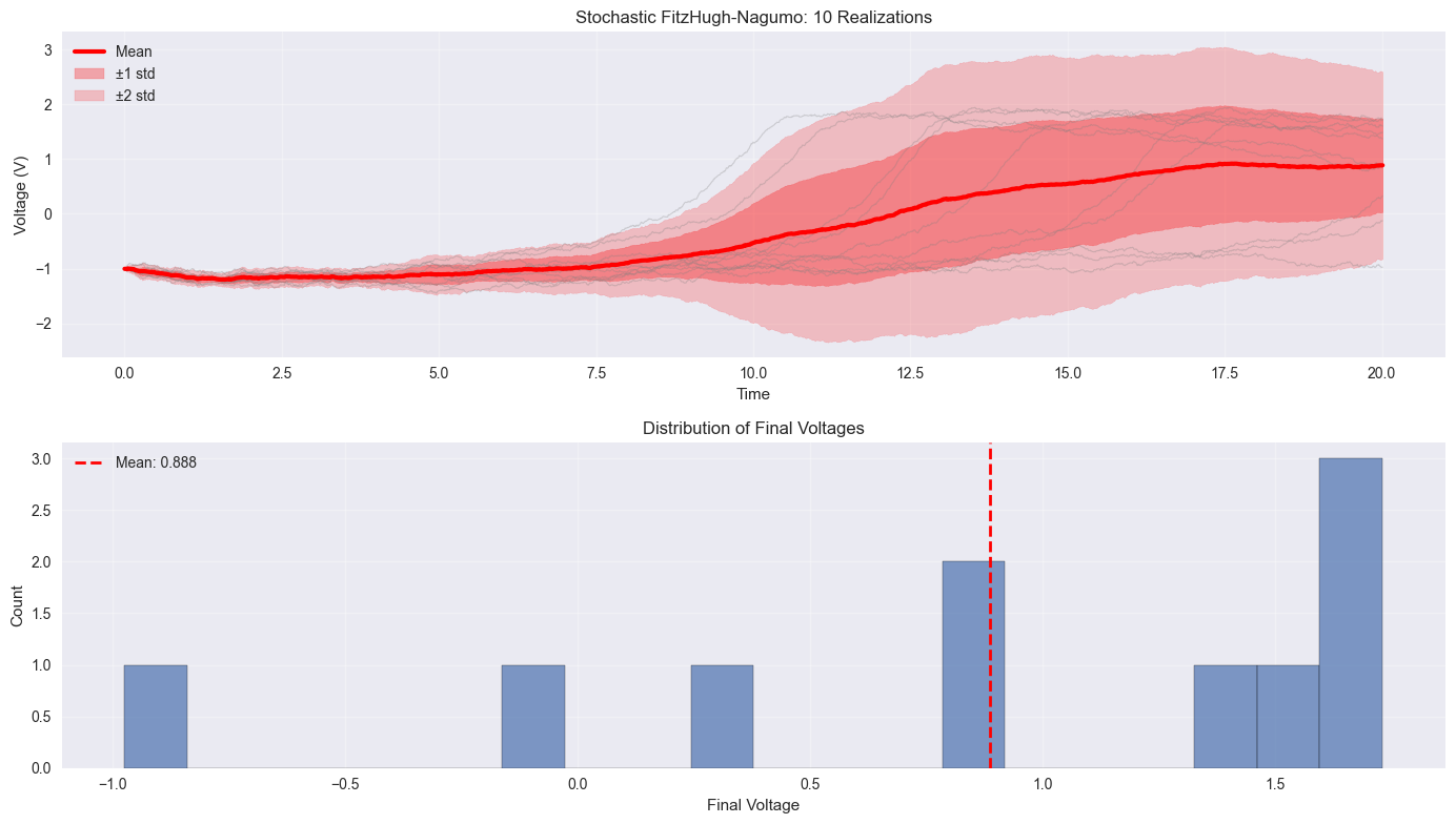
Statistics from 10 realizations:
Final voltage - Mean: 0.8878, Std: 0.8540
Final voltage - Min: -0.9736, Max: 1.7321

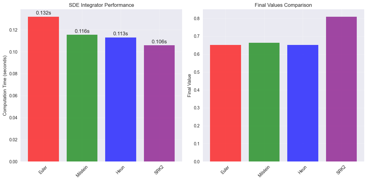
7. Performance Comparison

Let’s compare the computational efficiency of different SDE integrators:

import time


# Timing test setup for SDEs
def time_sde_integrator(integrator_func, df, dg, y0, n_steps, dt_val, *args, **kwargs):
    """Time an SDE integrator over n_steps"""
    t_array_timing = jnp.arange(0, n_steps * dt_val, dt_val)

    # Warm-up run (for JAX compilation)
    _ = integrate_sde(integrator_func, df, dg, y0, t_array_timing[:10], *args, **kwargs)

    # Actual timing
    start_time = time.time()
    result = integrate_sde(integrator_func, df, dg, y0, t_array_timing, *args, **kwargs)
    end_time = time.time()

    return end_time - start_time, result[-1]


# Timing parameters
n_steps_timing = 1000
dt_timing = 0.01

timing_methods = {
    'Euler': (braintools.quad.sde_euler_step, {}),
    'Milstein': (braintools.quad.sde_milstein_step, {'sde_type': 'ito'}),
    'Heun': (braintools.quad.sde_heun_step, {'sde_type': 'ito'}),
    'SRK2': (braintools.quad.sde_srk2_step, {}),
}

times = {}
final_values = {}

print(f"Timing SDE integrators over {n_steps_timing} steps...")
for name, (method, kwargs) in timing_methods.items():
    brainstate.random.set_key(jax.random.PRNGKey(42))  # Same seed for all
    elapsed, final_val = time_sde_integrator(
        method, gbm_drift, gbm_diffusion, y0, n_steps_timing, dt_timing,
        mu, sigma, **kwargs
    )
    times[name] = elapsed
    final_values[name] = final_val
    print(f"{name:10s}: {elapsed:.4f} seconds, final value: {final_val:.6f}")

# Efficiency analysis
euler_time = times['Euler']
print("\nRelative timing (vs Euler-Maruyama):")
for name, time_val in times.items():
    print(f"{name:10s}: {time_val / euler_time:.2f}x")

# Create performance visualization
plt.figure(figsize=(12, 6))

plt.subplot(1, 2, 1)
methods_list = list(times.keys())
times_list = [times[name] for name in methods_list]
bars = plt.bar(methods_list, times_list, alpha=0.7,
               color=['red', 'green', 'blue', 'purple'])
plt.ylabel('Computation Time (seconds)')
plt.title('SDE Integrator Performance')
plt.xticks(rotation=45)
plt.grid(True, alpha=0.3)

# Add value labels on bars
for bar, time_val in zip(bars, times_list):
    plt.text(bar.get_x() + bar.get_width() / 2, bar.get_height() + 0.001,
             f'{time_val:.3f}s', ha='center', va='bottom')

plt.subplot(1, 2, 2)
final_vals = [final_values[name] for name in methods_list]
plt.bar(methods_list, final_vals, alpha=0.7,
        color=['red', 'green', 'blue', 'purple'])
plt.ylabel('Final Value')
plt.title('Final Values Comparison')
plt.xticks(rotation=45)
plt.grid(True, alpha=0.3)

plt.tight_layout()
plt.show()

Timing SDE integrators over 1000 steps...
Euler     : 0.1320 seconds, final value: 0.651900
Milstein  : 0.1155 seconds, final value: 0.662962
Heun      : 0.1132 seconds, final value: 0.651795
SRK2      : 0.1059 seconds, final value: 0.809137

Relative timing (vs Euler-Maruyama):
Euler     : 1.00x
Milstein  : 0.87x
Heun      : 0.86x
SRK2      : 0.80x

Summary

This tutorial covered the key SDE integrators available in BrainTools:

Basic Methods:

• Euler-Maruyama: Simple, strong order 0.5, weak order 1.0

• Milstein: Higher accuracy with strong order 1.0

• Exponential Euler: Better stability for stiff SDEs

Advanced Methods:

• Stochastic Heun: Predictor-corrector scheme

• Tamed Euler: Prevents explosion for superlinear growth

• Implicit Euler: Enhanced stability via fixed-point iteration

• SRK methods: Stochastic Runge-Kutta for Stratonovich SDEs

Key Concepts:

• Itô vs Stratonovich: Different stochastic calculus interpretations

• Strong vs Weak convergence: Different measures of accuracy

• Noise handling: All methods use brainstate.random for Gaussian noise

Guidelines:

1. For most problems: Use Euler-Maruyama or Milstein

2. For higher accuracy: Use Milstein (strong order 1.0)

3. For stiff problems: Try Exponential Euler or Tamed Euler

4. For superlinear growth: Use Tamed Euler

5. For Stratonovich SDEs: Consider SRK methods

BrainTools Features:

• All methods work with JAX PyTrees

• Global time step management via brainstate.environ

• Consistent random number handling via brainstate.random

• Support for both Itô and Stratonovich interpretations

• Unit-aware computations with brainunit

Choose your SDE integrator based on the trade-off between accuracy, stability, and computational cost for your specific stochastic system.