Tutorial 1: Basic Connectivity Patterns

This tutorial introduces the fundamental connectivity patterns in braintools.conn. You’ll learn how to create basic network topologies, understand connection results, and work with weights and delays.

---

1. Introduction to Connectivity

Neural networks are defined not just by their neurons, but by how those neurons are connected. The braintools.conn module provides a comprehensive system for generating biologically-plausible connectivity patterns.

Why Connectivity Matters

• Network Dynamics: Connection patterns determine how information flows through neural populations

• Computational Properties: Different topologies enable different computations

• Biological Realism: Real neural circuits exhibit specific connectivity motifs

• Efficiency: Sparse connectivity reduces computational cost while maintaining function

Let’s start by importing the necessary libraries:

import numpy as np
import matplotlib.pyplot as plt
import brainunit as u
from braintools import conn, visualize as vis
from braintools.init import Constant, Normal, Uniform, LogNormal

# Set random seed for reproducibility
np.random.seed(42)

# Configure matplotlib
plt.rcParams['figure.figsize'] = (12, 4)
plt.rcParams['font.size'] = 10

print("✓ Imports successful")

✓ Imports successful

---

2. Understanding ConnectionResult

All connectivity patterns in braintools.conn return a ConnectionResult object. This object contains:

• pre_indices: Array of presynaptic neuron indices

• post_indices: Array of postsynaptic neuron indices

• weights: Synaptic weights (optional)

• delays: Synaptic delays (optional)

• metadata: Additional information about the connectivity pattern

Let’s create a simple connection and examine its structure:

# Create a simple random connectivity
simple_conn = conn.Random(prob=0.1, seed=42)
result = simple_conn(pre_size=10, post_size=10)

print("ConnectionResult Structure:")
print("=" * 50)
print(f"Number of connections: {len(result.pre_indices)}")
print(f"\nPresynaptic indices (first 10):")
print(result.pre_indices[:10])
print(f"\nPostsynaptic indices (first 10):")
print(result.post_indices[:10])
print(f"\nWeights: {result.weights}")
print(f"Delays: {result.delays}")
print(f"\nMetadata:")
for key, value in result.metadata.items():
    print(f"  {key}: {value}")

ConnectionResult Structure:
==================================================
Number of connections: 12

Presynaptic indices (first 10):
[0 1 3 3 4 4 6 6 7 8]

Postsynaptic indices (first 10):
[7 2 2 6 1 7 2 4 5 0]

Weights: None
Delays: None

Metadata:
  pattern: random
  probability: 0.1
  allow_self_connections: False
  weight_initialization: None
  delay_initialization: None

Connection Density

Let’s calculate the connection density (ratio of actual connections to possible connections):

def calculate_density(result, allow_self_connections=False):
    """Calculate connection density from ConnectionResult."""
    pre_size = result.pre_size if isinstance(result.pre_size, int) else np.prod(result.pre_size)
    post_size = result.post_size if isinstance(result.post_size, int) else np.prod(result.post_size)
    
    max_connections = pre_size * post_size
    if not allow_self_connections and pre_size == post_size:
        max_connections -= pre_size
    
    actual_connections = len(result.pre_indices)
    density = actual_connections / max_connections
    
    return density, actual_connections, max_connections

density, actual, maximum = calculate_density(result)
print(f"Connection density: {density:.1%}")
print(f"Actual connections: {actual} / {maximum} possible")
print(f"Expected density (prob=0.1): ~10%")

Connection density: 13.3%
Actual connections: 12 / 90 possible
Expected density (prob=0.1): ~10%

---

3. Random Connectivity

Random connectivity is the simplest and most fundamental pattern. Each potential connection is made with a fixed probability.

3.1 Basic Random Connectivity

The Random class (also aliased as FixedProb) creates connections with a specified probability:

# Create random connectivity with 10% connection probability
random_conn = conn.Random(prob=0.1, seed=42)
result_random = random_conn(pre_size=100, post_size=100)

print(f"Random Connectivity (prob=0.1)")
print(f"Generated {len(result_random.pre_indices)} connections")

density, actual, maximum = calculate_density(result_random)
print(f"Connection density: {density:.2%}")
print(f"Expected: ~10%")

Random Connectivity (prob=0.1)
Generated 1019 connections
Connection density: 10.29%
Expected: ~10%

3.2 Effect of Connection Probability

Let’s examine how connection probability affects network density:

# Test different probabilities
probabilities = [0.01, 0.05, 0.1, 0.2, 0.3, 0.5]
network_size = 100

results_by_prob = {}
for prob in probabilities:
    conn_pattern = conn.Random(prob=prob, seed=42)
    result = conn_pattern(pre_size=network_size, post_size=network_size)
    density, n_conn, _ = calculate_density(result)
    results_by_prob[prob] = (n_conn, density)

# Display results
print("\nConnection Probability vs. Actual Density:")
print("=" * 60)
print(f"{'Probability':<15} {'Connections':<15} {'Density':<15} {'Error'}")
print("=" * 60)
for prob in probabilities:
    n_conn, density = results_by_prob[prob]
    error = abs(density - prob) / prob * 100
    print(f"{prob:<15.2f} {n_conn:<15} {density:<15.4f} {error:>5.1f}%")

Connection Probability vs. Actual Density:
============================================================
Probability     Connections     Density         Error
============================================================
0.01            93              0.0094            6.1%
0.05            486             0.0491            1.8%
0.10            1019            0.1029            2.9%
0.20            2021            0.2041            2.1%
0.30            3021            0.3052            1.7%
0.50            5021            0.5072            1.4%

3.3 Self-Connections

By default, self-connections (neuron connecting to itself) are disabled. Let’s see the difference:

# Without self-connections (default)
conn_no_self = conn.Random(prob=0.2, allow_self_connections=False, seed=42)
result_no_self = conn_no_self(pre_size=50, post_size=50)

# With self-connections
conn_with_self = conn.Random(prob=0.2, allow_self_connections=True, seed=42)
result_with_self = conn_with_self(pre_size=50, post_size=50)

# Check for self-connections
self_conn_mask = result_with_self.pre_indices == result_with_self.post_indices
n_self_connections = np.sum(self_conn_mask)

print("Self-Connections Comparison:")
print("=" * 50)
print(f"Without self-connections: {len(result_no_self.pre_indices)} connections")
print(f"With self-connections:    {len(result_with_self.pre_indices)} connections")
print(f"Number of self-connections: {n_self_connections}")
print(f"Expected self-connections: ~{50 * 0.2:.1f} (50 neurons × 20% prob)")

Self-Connections Comparison:
==================================================
Without self-connections: 519 connections
With self-connections:    524 connections
Number of self-connections: 9
Expected self-connections: ~10.0 (50 neurons × 20% prob)

---

4. Regular Deterministic Patterns

In addition to random connectivity, braintools.conn provides deterministic connectivity patterns.

4.1 All-to-All Connectivity

The AllToAll pattern connects every presynaptic neuron to every postsynaptic neuron:

# Create all-to-all connectivity
all2all = conn.AllToAll(include_self_connections=False)
result_all2all = all2all(pre_size=10, post_size=10)

print("All-to-All Connectivity:")
print("=" * 50)
print(f"Network size: 10 × 10")
print(f"Connections: {len(result_all2all.pre_indices)}")
print(f"Expected: 10 × 10 - 10 (self) = 90")

density, _, _ = calculate_density(result_all2all)
print(f"Density: {density:.1%}")

All-to-All Connectivity:
==================================================
Network size: 10 × 10
Connections: 90
Expected: 10 × 10 - 10 (self) = 90
Density: 100.0%

4.2 One-to-One Connectivity

The OneToOne pattern creates one-to-one mappings, useful for identity mappings or layer-to-layer projections:

# Equal sizes
one2one_equal = conn.OneToOne()
result_equal = one2one_equal(pre_size=10, post_size=10)

print("One-to-One Connectivity (Equal Sizes):")
print("=" * 50)
print(f"Pre size: 10, Post size: 10")
print(f"Connections: {len(result_equal.pre_indices)}")
print(f"Connection pairs (pre → post):")
for i in range(min(5, len(result_equal.pre_indices))):
    print(f"  {result_equal.pre_indices[i]} → {result_equal.post_indices[i]}")

# Different sizes (non-circular)
one2one_diff = conn.OneToOne(circular=False)
result_diff = one2one_diff(pre_size=8, post_size=12)

print(f"\nOne-to-One Connectivity (Different Sizes, Non-Circular):")
print("=" * 50)
print(f"Pre size: 8, Post size: 12")
print(f"Connections: {len(result_diff.pre_indices)}")
print(f"Note: Only first 8 neurons connected (min of 8 and 12)")

# Circular mapping
one2one_circ = conn.OneToOne(circular=True)
result_circ = one2one_circ(pre_size=8, post_size=12)

print(f"\nOne-to-One Connectivity (Different Sizes, Circular):")
print("=" * 50)
print(f"Pre size: 8, Post size: 12")
print(f"Connections: {len(result_circ.pre_indices)}")
print(f"Connection pairs (pre → post):")
for i in range(min(12, len(result_circ.pre_indices))):
    print(f"  {result_circ.pre_indices[i]} → {result_circ.post_indices[i]}")
print(f"Note: Pre indices wrap around using modulo (% 8)")

One-to-One Connectivity (Equal Sizes):
==================================================
Pre size: 10, Post size: 10
Connections: 10
Connection pairs (pre → post):
  0 → 0
  1 → 1
  2 → 2
  3 → 3
  4 → 4

One-to-One Connectivity (Different Sizes, Non-Circular):
==================================================
Pre size: 8, Post size: 12
Connections: 8
Note: Only first 8 neurons connected (min of 8 and 12)

One-to-One Connectivity (Different Sizes, Circular):
==================================================
Pre size: 8, Post size: 12
Connections: 12
Connection pairs (pre → post):
  0 → 0
  1 → 1
  2 → 2
  3 → 3
  4 → 4
  5 → 5
  6 → 6
  7 → 7
  0 → 8
  1 → 9
  2 → 10
  3 → 11
Note: Pre indices wrap around using modulo (% 8)

---

5. Working with Weights and Delays

Synaptic weights and delays are crucial for realistic neural network simulations. braintools.conn supports flexible initialization through the braintools.init module.

5.1 Constant Weights and Delays

The simplest approach uses constant values with physical units:

# Random connectivity with constant weights and delays
conn_const = conn.Random(
    prob=0.1,
    weight=Constant(1.5 * u.nS),  # Synaptic conductance
    delay=Constant(2.0 * u.ms),   # Transmission delay
    seed=42
)

result_const = conn_const(pre_size=50, post_size=50)

print("Connectivity with Constant Weights and Delays:")
print("=" * 50)
print(f"Number of connections: {len(result_const.pre_indices)}")
print(f"\nWeight statistics:")
print(f"  Mean: {np.mean(result_const.weights)}")
print(f"  Std:  {np.std(result_const.weights)}")
print(f"  All weights are identical: {np.all(result_const.weights == result_const.weights[0])}")
print(f"\nDelay statistics:")
print(f"  Mean: {np.mean(result_const.delays)}")
print(f"  Std:  {np.std(result_const.delays)}")

Connectivity with Constant Weights and Delays:
==================================================
Number of connections: 263

Weight statistics:
  Mean: 1.5 * nsiemens
  Std:  0.0 * nsiemens
  All weights are identical: True

Delay statistics:
  Mean: 2.0 * msecond
  Std:  0.0 * msecond

5.2 Stochastic Weight Distributions

More realistic networks use stochastic weight distributions:

Normal Distribution

# Normal (Gaussian) distribution
conn_normal = conn.Random(
    prob=0.15,
    weight=Normal(mean=1.0 * u.nS, std=0.2 * u.nS),
    delay=Normal(mean=1.5 * u.ms, std=0.3 * u.ms),
    seed=42
)

result_normal = conn_normal(pre_size=100, post_size=100)

print("Normal Distribution Weights and Delays:")
print("=" * 50)
print(f"Number of connections: {len(result_normal.pre_indices)}")
print(f"\nWeight statistics:")
print(f"  Mean: {np.mean(result_normal.weights):.3f}")
print(f"  Std:  {np.std(result_normal.weights):.3f}")
print(f"  Min:  {np.min(result_normal.weights):.3f}")
print(f"  Max:  {np.max(result_normal.weights):.3f}")
print(f"\nDelay statistics:")
print(f"  Mean: {np.mean(result_normal.delays):.3f}")
print(f"  Std:  {np.std(result_normal.delays):.3f}")
print(f"  Min:  {np.min(result_normal.delays):.3f}")
print(f"  Max:  {np.max(result_normal.delays):.3f}")

Normal Distribution Weights and Delays:
==================================================
Number of connections: 1515

Weight statistics:
  Mean: 1.004 * nsiemens
  Std:  0.201 * nsiemens
  Min:  0.233 * nsiemens
  Max:  1.675 * nsiemens

Delay statistics:
  Mean: 1.493 * msecond
  Std:  0.291 * msecond
  Min:  0.323 * msecond
  Max:  2.374 * msecond

Uniform Distribution

# Uniform distribution
conn_uniform = conn.Random(
    prob=0.15,
    weight=Uniform(low=0.5 * u.nS, high=2.0 * u.nS),
    delay=Uniform(low=0.5 * u.ms, high=3.0 * u.ms),
    seed=42
)

result_uniform = conn_uniform(pre_size=100, post_size=100)

print("Uniform Distribution Weights and Delays:")
print("=" * 50)
print(f"Weight range: [0.5, 2.0] nS")
print(f"  Mean: {np.mean(result_uniform.weights):.3f}")
print(f"  Std:  {np.std(result_uniform.weights):.3f}")
print(f"  Min:  {np.min(result_uniform.weights):.3f}")
print(f"  Max:  {np.max(result_uniform.weights):.3f}")
print(f"\nDelay range: [0.5, 3.0] ms")
print(f"  Mean: {np.mean(result_uniform.delays):.3f}")
print(f"  Std:  {np.std(result_uniform.delays):.3f}")
print(f"  Min:  {np.min(result_uniform.delays):.3f}")
print(f"  Max:  {np.max(result_uniform.delays):.3f}")

Uniform Distribution Weights and Delays:
==================================================
Weight range: [0.5, 2.0] nS
  Mean: 1.258 * nsiemens
  Std:  0.432 * nsiemens
  Min:  0.500 * nsiemens
  Max:  2.000 * nsiemens

Delay range: [0.5, 3.0] ms
  Mean: 1.749 * msecond
  Std:  0.729 * msecond
  Min:  0.500 * msecond
  Max:  2.998 * msecond

Log-Normal Distribution

Log-normal distributions are common in biological synaptic weights:

# Log-normal distribution (common in biological synapses)
conn_lognormal = conn.Random(
    prob=0.15,
    weight=LogNormal(mean=1.0 * u.nS, std=0.5 * u.nS),
    delay=Constant(1.0 * u.ms),
    seed=42
)

result_lognormal = conn_lognormal(pre_size=100, post_size=100)

print("Log-Normal Distribution Weights:")
print("=" * 50)
print(f"Weight statistics:")
print(f"  Mean: {np.mean(result_lognormal.weights):.3f}")
print(f"  Std:  {np.std(result_lognormal.weights):.3f}")
print(f"  Median: {u.math.median(result_lognormal.weights):.3f}")
print(f"  Min:  {np.min(result_lognormal.weights):.3f}")
print(f"  Max:  {np.max(result_lognormal.weights):.3f}")
print(f"\nNote: Log-normal has positive skew (long tail)")

Log-Normal Distribution Weights:
==================================================
Weight statistics:
  Mean: 1.011 * nsiemens
  Std:  0.507 * nsiemens
  Median: 0.898 * nsiemens
  Min:  0.146 * nsiemens
  Max:  4.410 * nsiemens

Note: Log-normal has positive skew (long tail)

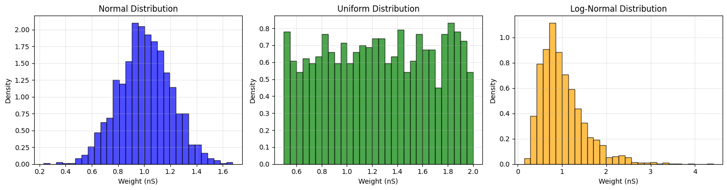
5.3 Visualizing Weight Distributions

Let’s compare the different weight distributions visually using braintools.visualize:

# Extract weight values (remove units for plotting)
weights_normal = u.get_mantissa(result_normal.weights)
weights_uniform = u.get_mantissa(result_uniform.weights)
weights_lognormal = u.get_mantissa(result_lognormal.weights)

# Create figure with subplots
fig, axes = plt.subplots(1, 3, figsize=(15, 4))

# Plot each distribution using vis.distribution_plot
vis.distribution_plot(
    weights_normal,
    bins=30,
    alpha=0.7,
    colors=['blue'],
    edgecolor='black',
    ax=axes[0],
    xlabel='Weight (nS)',
    title='Normal Distribution'
)

vis.distribution_plot(
    weights_uniform,
    bins=30,
    alpha=0.7,
    colors=['green'],
    edgecolor='black',
    ax=axes[1],
    xlabel='Weight (nS)',
    title='Uniform Distribution'
)

vis.distribution_plot(
    weights_lognormal,
    bins=30,
    alpha=0.7,
    colors=['orange'],
    edgecolor='black',
    ax=axes[2],
    xlabel='Weight (nS)',
    title='Log-Normal Distribution'
)

plt.tight_layout()
plt.show()

print("\nKey Observations:")
print("- Normal: Symmetric around mean")
print("- Uniform: Flat distribution within range")
print("- Log-Normal: Right-skewed with long tail (biologically realistic)")

Key Observations:
- Normal: Symmetric around mean
- Uniform: Flat distribution within range
- Log-Normal: Right-skewed with long tail (biologically realistic)

---

6. Visualizing Connectivity

Visualization helps us understand connectivity patterns. We’ll use braintools.visualize for professional-quality plots.

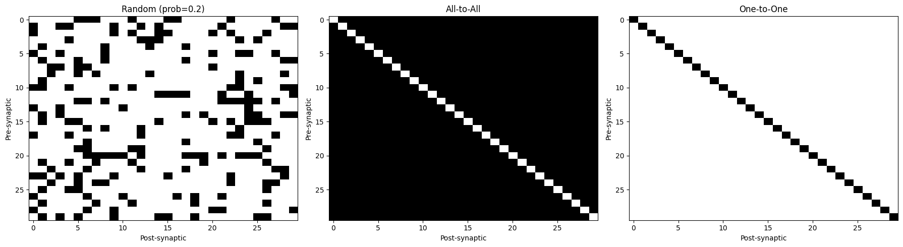
6.1 Connectivity Matrix

A connectivity matrix shows which neurons connect to which. We’ll use vis.connectivity_matrix():

def result_to_matrix(result):
    """Convert ConnectionResult to connectivity matrix."""
    pre_size = result.pre_size if isinstance(result.pre_size, int) else int(np.prod(result.pre_size))
    post_size = result.post_size if isinstance(result.post_size, int) else int(np.prod(result.post_size))
    
    conn_matrix = np.zeros((pre_size, post_size))
    conn_matrix[result.pre_indices, result.post_indices] = 1
    
    return conn_matrix

# Compare different patterns
conn_patterns = [
    (conn.Random(prob=0.2, seed=42), "Random (prob=0.2)"),
    (conn.AllToAll(include_self_connections=False), "All-to-All"),
    (conn.OneToOne(), "One-to-One"),
]

fig, axes = plt.subplots(1, 3, figsize=(18, 5))

for idx, (conn_pattern, name) in enumerate(conn_patterns):
    result = conn_pattern(pre_size=30, post_size=30)
    conn_mat = result_to_matrix(result)
    
    vis.connectivity_matrix(
        conn_mat,
        cmap='binary',
        center_zero=False,
        show_colorbar=False,
        ax=axes[idx],
        title=name
    )

plt.tight_layout()
plt.show()

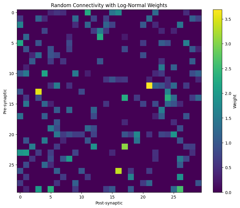
6.2 Weight Matrix Visualization

When weights are present, we can visualize their distribution in the connectivity matrix:

# Create connectivity with weights
conn_weighted = conn.Random(
    prob=0.2,
    weight=LogNormal(mean=1.0 * u.nS, std=0.6 * u.nS),
    seed=42
)
result_weighted = conn_weighted(pre_size=30, post_size=30)

# Create weight matrix
pre_size = 30
post_size = 30
weight_matrix = np.zeros((pre_size, post_size))
weights = u.get_mantissa(result_weighted.weights)
weight_matrix[result_weighted.pre_indices, result_weighted.post_indices] = weights

# Plot using vis.connectivity_matrix
fig, ax = plt.subplots(figsize=(10, 8))
vis.connectivity_matrix(
    weight_matrix,
    cmap='viridis',
    center_zero=False,
    show_colorbar=True,
    ax=ax,
    title='Random Connectivity with Log-Normal Weights'
)
plt.show()

6.3 Degree Distribution

The degree distribution shows how many connections each neuron has:

# Test with random connectivity
conn_test = conn.Random(prob=0.15, seed=42)
result_test = conn_test(pre_size=200, post_size=200)

# Calculate degrees
pre_size = 200
post_size = 200
out_degree = np.bincount(result_test.pre_indices, minlength=pre_size)
in_degree = np.bincount(result_test.post_indices, minlength=post_size)

# Plot using vis.distribution_plot
fig, axes = plt.subplots(1, 2, figsize=(14, 5))

vis.distribution_plot(
    out_degree,
    bins=20,
    alpha=0.7,
    colors=['blue'],
    edgecolor='black',
    ax=axes[0],
    xlabel='Out-Degree (outgoing connections)',
    ylabel='Count',
    title='Out-Degree Distribution'
)

vis.distribution_plot(
    in_degree,
    bins=20,
    colors=['green'],
    edgecolor='black',
    alpha=0.7,
    ax=axes[1],
    xlabel='In-Degree (incoming connections)',
    ylabel='Count',
    title='In-Degree Distribution'
)

plt.suptitle('Random Connectivity (prob=0.15)', fontsize=14, y=1.02)
plt.tight_layout()
plt.show()

print(f"Out-degree: mean={np.mean(out_degree):.2f}, std={np.std(out_degree):.2f}")
print(f"In-degree:  mean={np.mean(in_degree):.2f}, std={np.std(in_degree):.2f}")

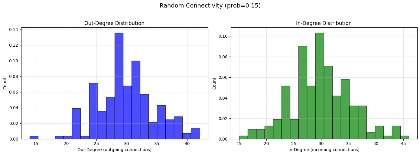
Out-degree: mean=29.86, std=4.74
In-degree:  mean=29.86, std=5.55

6.4 Advanced Visualization: Correlation Matrix

Let’s visualize correlations between neurons’ connectivity patterns:

# Create a network with some structure
conn_struct = conn.Random(prob=0.15, seed=42)
result_struct = conn_struct(pre_size=50, post_size=50)

# Create connectivity matrix
conn_mat = result_to_matrix(result_struct)

# Sample subset for visualization clarity
subset_size = 20
conn_subset = conn_mat[:subset_size, :subset_size]

# Plot correlation matrix
fig, ax = plt.subplots(figsize=(10, 8))
vis.correlation_matrix(
    conn_subset,
    method='pearson',
    cmap='RdBu_r',
    show_values=False,
    ax=ax,
    title='Connectivity Pattern Correlation (20×20 subset)'
)
plt.show()

print("\nThis shows correlations between neurons' connectivity patterns.")
print("High correlation means neurons have similar connection patterns.")

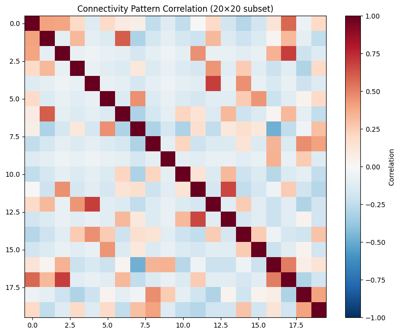
This shows correlations between neurons' connectivity patterns.
High correlation means neurons have similar connection patterns.

---

7. Exercises

Try these exercises to reinforce your understanding:

Exercise 1: Connection Probability Calibration

Create a function that finds the connection probability needed to achieve a target number of connections:

def find_target_probability(pre_size, post_size, target_connections, tolerance=50, max_iterations=20):
    """
    Find connection probability to achieve target number of connections.
    
    Parameters
    ----------
    pre_size : int
        Number of presynaptic neurons
    post_size : int
        Number of postsynaptic neurons
    target_connections : int
        Desired number of connections
    tolerance : int
        Acceptable deviation from target
    max_iterations : int
        Maximum search iterations
    
    Returns
    -------
    prob : float
        Connection probability
    actual : int
        Actual connections achieved
    """
    # YOUR CODE HERE
    # Hint: Use binary search or gradient descent approach
    # Start with initial probability estimate: target_connections / (pre_size * post_size)
    
    pass

# Test your function
# prob, actual = find_target_probability(pre_size=100, post_size=100, target_connections=1000)
# print(f"Target: 1000 connections")
# print(f"Probability: {prob:.4f}")
# print(f"Actual: {actual} connections")

Exercise 2: Weight Scaling

Create a custom weight initialization that scales weights inversely with the number of incoming connections (to maintain constant total input):

def create_scaled_weights(result, base_weight=1.0 * u.nS):
    """
    Scale weights inversely with in-degree to maintain constant total input.
    
    Parameters
    ----------
    result : ConnectionResult
        Connectivity result
    base_weight : Quantity
        Base weight value
    
    Returns
    -------
    scaled_weights : array
        Scaled weight array
    """
    # YOUR CODE HERE
    # Hint: Calculate in-degree for each post neuron
    # Then scale weights: w_scaled = base_weight / in_degree
    
    pass

# Test your function
# conn_test = conn.Random(prob=0.1, seed=42)
# result_test = conn_test(pre_size=100, post_size=100)
# scaled_weights = create_scaled_weights(result_test, base_weight=1.0 * u.nS)
# 
# # Verify constant total input
# post_size = 100
# total_inputs = np.zeros(post_size)
# for post_idx in range(post_size):
#     mask = result_test.post_indices == post_idx
#     total_inputs[post_idx] = np.sum(u.get_mantissa(scaled_weights[mask]))
# 
# print(f"Total input per neuron - Mean: {np.mean(total_inputs):.3f}, Std: {np.std(total_inputs):.3f}")

Exercise 3: Connectivity Statistics

Write a function that computes comprehensive connectivity statistics:

def analyze_connectivity(result):
    """
    Compute comprehensive connectivity statistics.
    
    Should calculate:
    - Connection density
    - Mean/std of in-degree and out-degree
    - Weight statistics (if present)
    - Delay statistics (if present)
    - Reciprocal connections (if pre_size == post_size)
    
    Returns
    -------
    stats : dict
        Dictionary of statistics
    """
    # YOUR CODE HERE
    
    pass

# Test your function
# conn_test = conn.Random(prob=0.15, weight=Normal(mean=1.0*u.nS, std=0.2*u.nS), seed=42)
# result_test = conn_test(pre_size=100, post_size=100)
# stats = analyze_connectivity(result_test)
# 
# for key, value in stats.items():
#     print(f"{key}: {value}")